What is the difference between a blank row and a partially blank row?

A blank row contains no values in any relevant column. A partially blank row contains a record but is missing one or more fields. The $14 uncategorized receipt in this example is a partial record, so it must remain.

Why should I delete blank rows from the bottom upward?

Deleting a row changes the numbers of all rows beneath it. Removing the lowest target first preserves the original row numbers of the remaining targets.

What if column A can be blank in a valid record?

Don’t use `where A is not null` as the cleanup rule. Instead, choose a consistently populated field, such as a transaction ID, or inspect every relevant column to determine whether the entire row is empty.

Does QUERY delete the original rows?

No. `QUERY` generates a separate result and leaves `Transactions!A1:F13` unchanged. If you need a permanently cleaned copy, duplicate the tab and delete the entire blank rows there.

How to Delete Blank Rows in Google Sheets

If the source needs to remain unchanged, create a cleaned view with QUERY instead. Whichever method you choose, first distinguish completely blank rows from valid records with missing fields.

Identify completely blank rows

Use the synthetic workbook Spreadsheet formula and cleanup practice:

Use the Google Sheets copy for the native QUERY example. The XLSX companion provides the source data, guidance, and a portable SUM(F160:H160) example, but it doesn’t reproduce the native Google Sheets QUERY output.

Open Transactions!A1:F13. The columns are:

Column	Meaning
A	Date
B	Category
C	Description
D	Amount (USD)
E	Paid
F	Owner

This reference follows Google’s documented A1 notation.

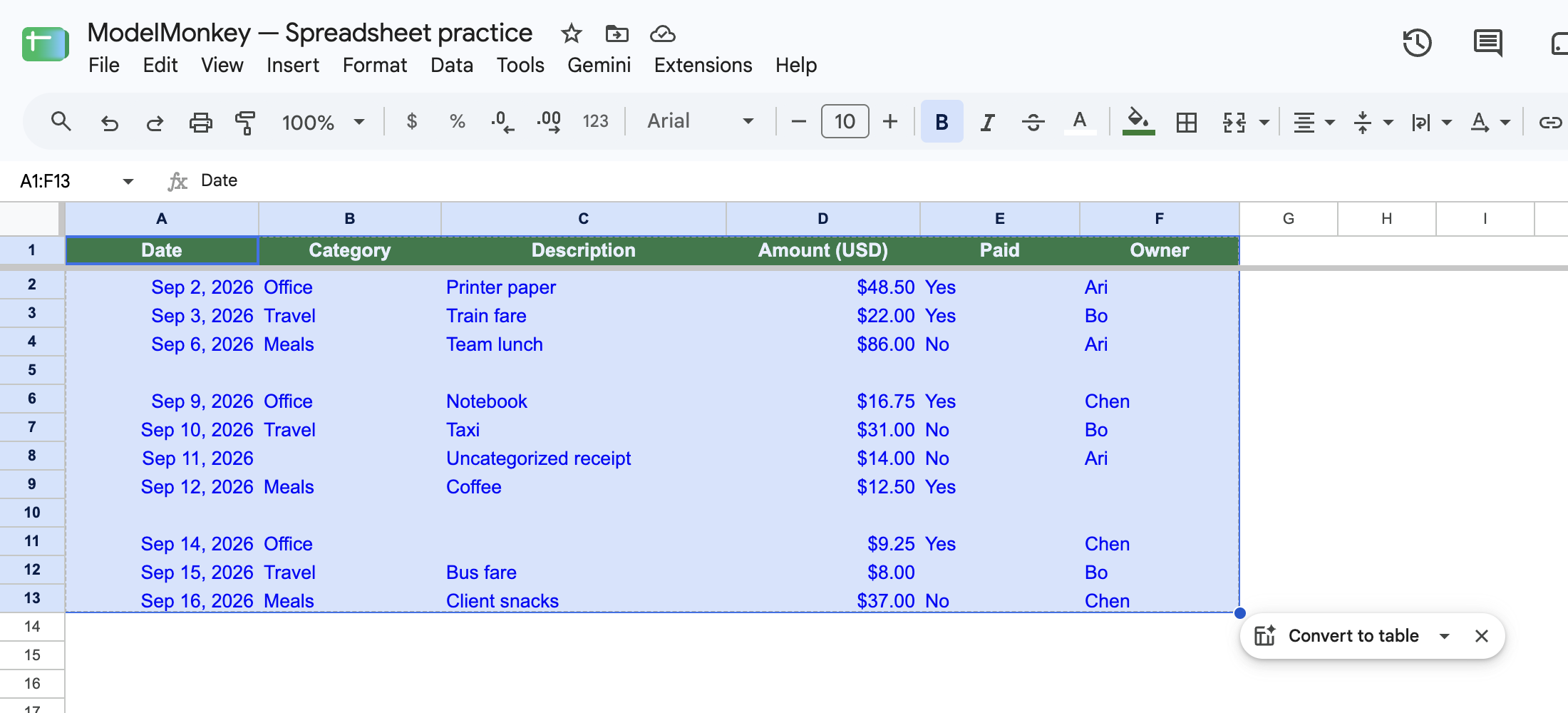
Spreadsheet formula and cleanup practice open in the actual Google Sheets interface with synthetic data

Actual Google Sheets screenshot of the restored synthetic example.

Rows 5 and 10 are blank across all 6 columns. They’re the only rows you should remove.

Other rows have missing fields but still contain valid records:

Source row	Missing field	Evidence that the record exists
8	Category	Date, description, $14 amount, payment status, and owner are populated
9	Owner	The other transaction fields contain data
11	Description	Date, category, amount, payment status, and owner are populated
12	Paid	The other transaction fields contain data

If you deleted every row containing an empty cell, you’d incorrectly remove these transactions.

Delete blank rows manually

First, duplicate the Transactions tab if you need to preserve the original. Because the template already includes a completed Cleanup result tab, name your duplicate Cleanup result - working.

Next, remove the 2 blank rows:

Click row number 10 to select the entire row.
Right-click and select Delete row.
Click row number 5.
Right-click and select Delete row again.

Start with row 10. If you delete row 5 first, the original row 10 moves to row 9, making it easier to delete the wrong record.

The recorded Google Sheets execution produced Cleanup result!A1:F11, with 1 header and 10 transaction records. To verify your result, compare the complete A1:F11 range with the source records after excluding only original rows 5 and 10.

You can also use these spot checks:

The populated range ends at row 11.
C7 contains Uncategorized receipt.
D7 contains 14 USD.

Together, these checks confirm that the partial record originally in row 8 remains. However, they don’t prove that every other valid record survived. For that, compare the entire cleaned range with the expected 10 records.

Avoid selecting a single empty cell and choosing a command that shifts cells upward. That action can move one field independently from the rest of its row and corrupt the record structure.

Create a clean view without deleting rows

If you want to retain the source exactly as received, enter this formula in Practice!A18:

=QUERY(Transactions!A1:F13,"select * where A is not null",1)

Here’s what each part does:

Transactions!A1:F13 specifies the source.
select * where A is not null retains rows where column A is nonblank.
1 identifies the first source row as the header.

Google documents this structure in its QUERY function reference. Depending on your spreadsheet locale, you may need semicolons instead of commas between the arguments.

In the recorded execution, the formula filled Practice!A18:F28 with 11 rows: the header plus all 10 transactions whose column A cells were populated. The result excluded the 2 wholly blank rows while retaining records with a missing Category, Description, Paid value, or Owner.

Keep in mind that the formula doesn’t verify whether column A contains a date. Text or any other nonblank value would also pass. This approach works for the example because every legitimate record has a date in column A. If a valid transaction might have an empty date, use a more reliable key, such as a transaction ID, or review the complete row before excluding it.

The recorded execution didn’t cover a source with no matching rows or cells that contain only whitespace. Because a visually empty cell may contain spaces or hidden characters, test those cases on a disposable copy before applying the formula to a recurring import.

Choose between deletion and QUERY

Requirement	Recommended method
Clean a copied export permanently	Delete entire rows manually
Preserve the raw source	Create a `QUERY` view
Keep records with some missing fields	Define the blank-row rule before using either method
No consistently populated key column	Review the whole row manually

For recurring finance imports, a separate clean view can be useful. Reporting formulas can reference the cleaned output while the original data remains available for reconciliation. For more examples, see how to use QUERY in Google Sheets for finance.

Ask ModelMonkey to clean the copied sheet

ModelMonkey can inspect Google Sheets context and help organize or change rows from a natural-language request. For this example, give it a specific instruction:

Duplicate the Transactions sheet as Cleanup result - working. On the duplicate, remove only rows where every cell from A through F is blank. Preserve any row containing at least one populated cell.

When the workflow presents a preview, review the proposed deletions before proceeding. Afterward, compare the complete resulting A1:F11 range with the expected 10 records. Then confirm that C7 equals Uncategorized receipt and D7 equals 14 USD.

Spreadsheet changes aren’t guaranteed to be correct, so always review the result. For more context, see AI assistance in Google Sheets for FP&A.