
=COUNTIF($D$15:$D$22,"*"&$B$4&"*")
With multiple criteria, first decide which result you need:
- ANY: Count each record once if it contains at least one active criterion.
- ALL: Count a record only if it contains every active criterion.
- Criterion hits: Count each criterion-record match. One record can contribute several hits, but repeated instances of the same criterion within that record still contribute only 1.
Adding several COUNTIF results produces criterion hits, not necessarily distinct records. To count distinct records, evaluate the matches row by row, then sum an ANY or ALL flag.
Download the example
The synthetic Excel COUNTIF Contains Multiple Criteria: Support Message Triage Template uses:
Keyword Triage!B4:B6forrefund,chargeback, andcancelKeyword Triage!B7for the optional exclusiontestKeyword Triage!B8for the active-keyword countKeyword Triage!A15:D26for ticket ID, received date, status, and messageKeyword Triage!E15:J26for match counts and audit flags
Copy this Google Sheets template or download the Excel file. The workbook contains the complete eight-record synthetic baseline used for the results below.

Enter the criteria in B4:B7, then use the adjacent summary to see how many records match.
Count cells containing one criterion
With messages in D15:D22 and refund in B4, enter:
=COUNTIF($D$15:$D$22,"*"&$B$4&"*")
The first * allows text before the criterion, while the second allows text after it. Microsoft documents the syntax and wildcard behavior in its COUNTIF function reference.
Standard COUNTIF text matching is case-insensitive, so refund, Refund, and REFUND all match. SEARCH is also case-insensitive, as documented in Microsoft’s SEARCH function reference.
Count criterion hits for multiple criteria
To add the counts for three criteria, use:
=SUM(COUNTIF($D$15:$D$22,{"*refund*","*chargeback*","*cancel*"}))
For the supplied eight-record baseline, the row match counts are:
1, 2, 2, 3, 0, 3, 1, 1
Their sum is 13 criterion hits, but only 7 distinct records contain at least one keyword. A record containing both refund and cancel contributes 2. If a message contains refund twice, it still contributes only 1 for that criterion because COUNTIF counts the matching cell, not each occurrence within it.
This formula works when you need the number of matching criterion-record pairs or know the criteria can’t overlap. Don’t use it to count distinct records when one message might contain several terms. For separate counts returned as an array, see Excel COUNTIF Array Criteria: Return Multiple Counts.
Count distinct records matching ANY criterion
For a distinct-record count, use a helper column to calculate how many active criteria each row contains.
Start by counting the nonblank keyword cells in B8:
=COUNTIF(B4:B6,"<>")
Next, count the criteria found in the message in D15 by entering this formula in E15:
=SUMPRODUCT(--($B$4:$B$6<>""),--ISNUMBER(SEARCH($B$4:$B$6,D15)))
Fill E15 through E26. The first condition ignores blank criteria. However, a cell containing only spaces isn’t blank, so Excel will treat it as an active search term.
Now create the raw ANY flag in F15:
=--(E15>0)
Fill the formula through F26, then calculate the distinct-record count:
=SUM(F15:F26)
The baseline result is 7. Each matching record contributes 1, no matter how many criteria it contains.
Count records matching ALL criteria
When all three keyword cells are populated, this COUNTIFS formula counts rows containing every criterion:
=COUNTIFS(
  $D$15:$D$22,"*"&$B$4&"*",
  $D$15:$D$22,"*"&$B$5&"*",
  $D$15:$D$22,"*"&$B$6&"*"
)
The baseline result is 2 because COUNTIFS applies every supplied condition to the same row. Microsoft documents its syntax in the COUNTIFS function reference.
If some keyword cells might be unused, the helper-column method handles them more reliably. Enter this formula in G15:
=--AND($B$8>0,E15=$B$8)
Fill it through G26, then sum the flags:
=SUM(G15:G26)
The B8>0 guard prevents an empty set of keywords from qualifying every row.
Exclude records containing another term
The example excludes messages containing test. To identify those records, enter this formula in H15:
=--AND($B$7<>"",ISNUMBER(SEARCH($B$7,D15)))
Fill it through H26. A value of 1 identifies an excluded record. When B7 is blank, the flag remains 0.
Next, combine the exclusion flag with raw ANY in I15:
=--AND(F15=1,H15=0)
For qualified ALL, enter this formula in J15:
=--AND(G15=1,H15=0)
Fill both formulas through row 26. Then calculate the qualified totals with:
=SUM(I15:I26)
=SUM(J15:J26)
The baseline workbook produces:
| Check | Result |
|---|---|
| Populated records | 8 |
| Raw ANY | 7 |
| Raw ALL | 2 |
Records containing test | 2 |
| Qualified ANY | 5 |
| Qualified ALL | 1 |
The counts reconcile as 7 raw ANY - 2 excluded = 5 qualified ANY.
Count qualified records by status
To count qualified ANY records whose status cell equals Open, use:
=COUNTIFS($C$15:$C$26,"Open",$I$15:$I$26,1)
For Escalated, use:
=COUNTIFS($C$15:$C$26,"Escalated",$I$15:$I$26,1)
These criteria use whole-cell equality, so a value such as Open - urgent won’t match Open. The comparison is case-insensitive, which means Open, open, and OPEN all match.
In the baseline, there are 2 Open and 2 Escalated qualified-ANY records. Records with other statuses still contribute to the overall qualified count.
If the case must also match, use EXACT:
=SUMPRODUCT(--EXACT($C$15:$C$26,"Open"),--($I$15:$I$26=1))
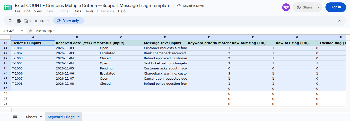
The record log shows why each message was included or excluded and how a newly entered message affects the summary.
Verify the formulas
The supplied Google Sheets test record covers the baseline, a changed criterion, an empty-keyword case, and a ninth record added in the first reserved row. Each check is independent, so restore the original eight-record baseline before starting the next one.
For an ongoing-use check, enter this record in A23:D23:
| Cell | Value |
|---|---|
| A23 | T-1009 |
| B23 | 2026-11-09 |
| C23 | Open |
| D23 | Please cancel and refund; chargeback not yet filed. |
The expected row result in E23:J23 is:
3, 1, 1, 0, 1, 1
The summary should become:
| Check | Expected result |
|---|---|
| Populated records | 9 |
| Raw ANY | 8 |
| Raw ALL | 3 |
| Qualified ANY | 6 |
| Qualified ALL | 2 |
| Open qualified ANY | 3 |
After you add the ninth record, the unused reserved rows E24:J26 display zero and don’t affect the summary.
Before running either boundary check below, clear A23:D23 to restore the original eight-record baseline:
- Replace
cancelinB6withinvoice. The expected results are 7 raw ANY, 0 raw ALL, 5 qualified ANY, 0 qualified ALL, 1 Open qualified ANY, and 2 Escalated qualified ANY. - Restore
cancelinB6, then clearB4:B6while leavingtestinB7.B8and every ANY, ALL, qualified, Open, and Escalated total should be 0. The two records containingtestcan still have exclusion flags because the exclusion is evaluated separately.
These tests were run in Google Sheets. After opening the XLSX file in Excel, recalculate it and compare the summary and several row flags with the documented results.
Common problems
Blank criteria: Clear unused keyword cells instead of entering placeholders such as N/A. Excel treats a placeholder as search text.
Whitespace-only criteria: A space isn’t blank. Remove it if the criterion should be inactive.
Duplicate counting: SUM(COUNTIF()) counts criterion-record matches. To count distinct records, use one row-level ANY flag.
Empty keyword set: Keep the B8>0 guard so the ALL logic returns 0 when no criteria are active.
Wildcards: ? matches one character, while * matches any sequence. To search for a literal question mark or asterisk, prefix it with a tilde, such as ~? or ~*.
Locale separators: These formulas use commas. Some Excel locales require semicolons.
Reserved rows: The template supports 12 records across rows 15:26. Replace data only in A15:D26, and leave E15:J26 intact.
Review the formula logic with ModelMonkey
ModelMonkey can inspect workbook context and help with formulas in Google Sheets and Excel. For this example, ask it to review B4:B8 and E15:J26, explain why an ANY or ALL count doesn’t reconcile, and propose a correction.
Before using a proposed change, check it against the row-level flags and expected totals.