
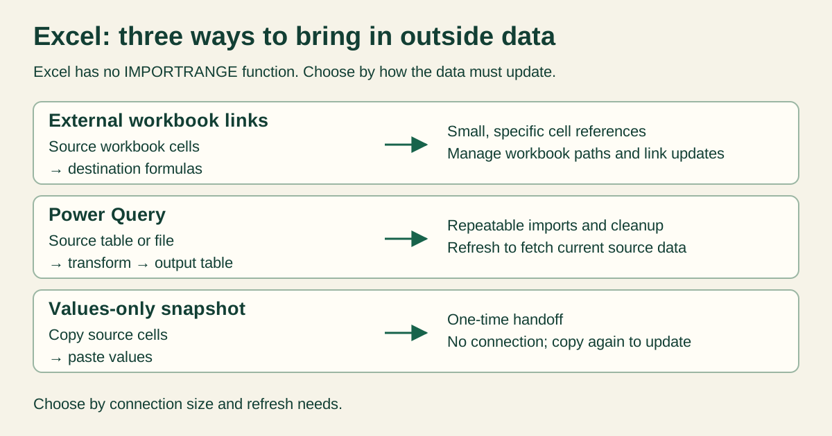
- Use an external workbook reference for a small number of linked cells.
- Use Power Query for a refreshable table that requires cleaning, transformation, or combination.
- Use copy-and-paste when you need a static snapshot.
For recurring FP&A schedules, Power Query is usually the most suitable option. Workbook links work well for individual assumptions or control figures.
Microsoft’s Excel function catalog doesn’t include an IMPORTRANGE function. Excel instead provides workbook links and Power Query data connections.
Reproducible finance example
This example imports departmental amounts from one Excel workbook into another.
Source workbook
- File:
C:\Finance\Budget_Source.xlsx - Worksheet:
Monthly_Data - Range:
A1:C4
| Cell | Date | Department | Amount_USD |
|---|---|---|---|
| Row 1 | Date | Department | Amount_USD |
| Row 2 | 2026-10-01 | Sales | 12500.00 |
| Row 3 | 2026-10-15 | Operations | 0.00 |
| Row 4 | 2026-10-31 | Sales | blank |
Enter dates as Excel date values, not text. Enter 12500.00 and 0.00 as numbers. Leave C4 genuinely empty.
Destination workbook
- File:
C:\Finance\Finance_Report.xlsx - Worksheets:
Linked_View,Query_View, andSnapshot_View
The expected imported result contains 3 data rows, a numeric total of 12500.00, one blank amount, and one numeric zero. These checks confirm that the transfer preserved the fixture. They don’t show whether the underlying budget is approved or accurate.
Method 1: Link cells to another Excel workbook
An external reference points a destination cell to a cell in another workbook. It’s a good choice for a small set of assumptions, KPIs, or control totals.
Open both workbooks, then enter these headers in Linked_View!A1:C1:
Date | Department | Amount_USD
Enter these formulas in row 2:
A2: =IF('[Budget_Source.xlsx]Monthly_Data'!A2="","",'[Budget_Source.xlsx]Monthly_Data'!A2)
B2: =IF('[Budget_Source.xlsx]Monthly_Data'!B2="","",'[Budget_Source.xlsx]Monthly_Data'!B2)
C2: =IF('[Budget_Source.xlsx]Monthly_Data'!C2="","",'[Budget_Source.xlsx]Monthly_Data'!C2)
Copy A2:C2 through row 4.
The IF wrapper matters because a bare external reference to an empty source cell can display 0. Returning "" preserves the intended blank in this example. If your Excel installation uses semicolons as formula separators, replace the commas with semicolons.
When the source workbook is closed, Excel may store the full file path:
=IF('C:\Finance\[Budget_Source.xlsx]Monthly_Data'!C2="","",'C:\Finance\[Budget_Source.xlsx]Monthly_Data'!C2)
Long paths are easy to mistype. Create the link by selecting the source cell instead of entering the reference manually.
Expected result
| Destination row | Date | Department | Amount_USD |
|---|---|---|---|
| 2 | 2026-10-01 | Sales | 12500.00 |
| 3 | 2026-10-15 | Operations | 0.00 |
| 4 | 2026-10-31 | Sales | blank |
The date display can vary with the workbook’s number format, but the underlying dates should remain unchanged.
Add these controls in Linked_View!E1:F4:
| Cell | Entry | Expected result |
|---|---|---|
| E1 | Loaded rows | |
| F1 | =COUNT(A2:A4) | 3 |
| E2 | Amount total | |
| F2 | =SUM(C2:C4) | 12500 |
| E3 | Blank amounts | |
| F3 | =COUNTBLANK(C2:C4) | 1 |
| E4 | Zero is numeric | |
| F4 | =AND(C3=0,ISNUMBER(C3)) | TRUE |
Workbook links can be updated, but they aren’t continuously synchronized database connections. Save changes in the source workbook, then update the destination through Excel’s workbook-link controls. Microsoft documents both current and older interfaces in Manage workbook links.
Method 2: Import the table with Power Query
Power Query is well suited to recurring schedules because it records the source, data types, and transformation steps in one query.
These instructions apply to desktop Excel for Windows:
- Save both workbooks.
- Open
Finance_Report.xlsx. - Select Data > Get Data > From File > From Excel Workbook.
- Select
C:\Finance\Budget_Source.xlsx. - In Navigator, select the
Monthly_Dataworksheet. - Select Transform Data.
- If the preview uses generic names such as
Column1, choose Use First Row as Headers once. Do not promote headers again ifDate,Department, andAmount_USDare already column names. - Set the column types:
Date: DateDepartment: TextAmount_USD: Decimal Number
- Do not add filters, duplicate removal, aggregation, or blank replacement.
- Select Home > Close & Load > Close & Load To.
- Choose Existing worksheet and enter
Query_View!$A$1. - Rename the resulting Excel table
tblImportedthrough Table Design > Table Name.
The expected output in Query_View!A1:C4 is the same 3-row fixture shown above. The final Amount_USD cell should remain blank, while the Operations amount should remain numeric zero.
Add these controls in Query_View!E1:F4:
| Cell | Entry | Expected result |
|---|---|---|
| E1 | Loaded rows | |
| F1 | =COUNT(tblImported[Date]) | 3 |
| E2 | Amount total | |
| F2 | =SUM(tblImported[Amount_USD]) | 12500 |
| E3 | Blank amounts | |
| F3 | =COUNTBLANK(tblImported[Amount_USD]) | 1 |
| E4 | Zero is numeric | |
| F4 | =AND(INDEX(tblImported[Amount_USD],2)=0,ISNUMBER(INDEX(tblImported[Amount_USD],2))) | TRUE |
After changing and saving the source, use Data > Refresh All or right-click the query table and select Refresh. Excel can also refresh certain connections when the destination workbook opens. See Microsoft’s external data refresh guidance.
Method 3: Create a static snapshot
Copy-and-paste is appropriate when the destination must remain fixed even if the source changes, such as for a controlled month-end snapshot.
- Copy
Monthly_Data!A1:C4. - Select
Snapshot_View!A1. - Choose Paste Special > Values.
- Format column A as dates and column C as currency or another appropriate numeric format.
Initially, the snapshot has the same 3 rows and 12500.00 total. If the source amount changes later, the pasted values remain unchanged. Use this method only when the snapshot is intended to stay static.
Which Excel IMPORTRANGE alternative should you use?
| Criterion | Workbook link | Power Query | Copy-and-paste |
|---|---|---|---|
| Best use | A few cells or assumptions | Recurring structured tables | Deliberate static snapshot |
| Update method | Recalculate or update workbook links | Refresh the query | Repeat the copy manually |
| Transform data | Limited to formulas | Supports defined transformation steps | None during the connection |
| Combine files | Impractical at scale | Designed for repeatable imports and combinations | Manual |
| Audit trail | Formulas show cell-level sources | Applied Steps show query logic | Limited unless source details are documented |
| Main maintenance risk | Broken or incorrect file references | Changed paths, credentials, columns, or types | Stale values |
| Blank handling | Must be handled in formulas | Blank values can remain null | Preserved as pasted |
| Duplicate handling | References whatever cells you specify | Duplicates remain unless a removal step is added | Duplicates remain |
For an FP&A model, a practical policy is:
- Use workbook links for a short list of assumptions or summary values.
- Use Power Query for transaction extracts, departmental schedules, and recurring data loads.
- Use values-only snapshots when a reporting period must no longer respond to source changes.
Acceptance tests to run
The following checks are proposed tests, not executed results. Run each one on a separate copy or restore the original fixture after each test.
| Test | Procedure | Expected result |
|---|---|---|
| Linked-view baseline | Recalculate Linked_View with both workbooks available. | 3 dates, Sales in B2, 12500.00 in C2, numeric zero in C3, and blank in C4. Controls return 3, 12500, 1, and TRUE. |
| Workbook-link update | Change Monthly_Data!C2 to 12750.00, save the source, and use Excel’s documented link-update command. | Linked_View!C2 becomes 12750.00; its amount total becomes 12750. |
| Moved source | Move Budget_Source.xlsx to another folder and reopen or update the destination. | Excel exposes an unresolved source link. Use the Workbook Links pane or the applicable Edit Links interface to select the new source. Do not replace formulas with zero. |
| Power Query baseline | Restore C2 to 12500.00 and refresh tblImported. | The query loads exactly 3 data rows. The dates, departments, numeric zero, and blank match the source. Controls return 3, 12500, 1, and TRUE. |
| Power Query refresh | Change Monthly_Data!C2 to 12750.00, save, and refresh the query. | The first amount becomes 12750.00; the other two rows remain unchanged. |
| Malformed amount | In a test copy, replace Monthly_Data!C2 with the text not-a-number and refresh. | The explicit Decimal Number step exposes a conversion error or reports a refresh error. The text must not silently become zero. |
| Empty source | In a test copy, retain only the source header row and refresh. | tblImported retains its headers and contains zero data rows. The loaded-row control returns 0. |
| Duplicate source row | Restore the fixture, duplicate row 2 exactly, and refresh. | Both copies remain because no deduplication step exists. The query has 4 rows and an amount total of 25000. Duplicate presence does not indicate approval or error. |
| Date boundaries | Inspect the first and last source dates after import. | Both 2026-10-01 and 2026-10-31 are present because the entire table is imported. There is no date-selection rule. |
| Static snapshot | Restore the original fixture, paste values into Snapshot_View, then change the source amount to 12750.00. | Snapshot_View remains at 12500.00 because it has no connection to the source. |
Enums, direction matching, opening entries, progress calculations, and paired transfers are outside this fixture. Adding that logic would require separate inputs and controls.
Fix broken links and refresh failures
The source file was moved or renamed
A workbook link stores a source location. Use Excel’s Workbook Links controls to point it to the new file.
Power Query also retains the source path. Open the query, inspect its Source step, and select the replacement file. Then refresh and rerun the row, total, blank, and numeric-zero controls.
The user cannot access the source
Having a valid path isn’t enough if the user lacks access to the file or folder. Confirm that the source can be opened under the same account used for the refresh. For remote sources, review the query’s data-source credentials instead of bypassing Excel’s security prompts.
The source changed but the destination did not
First, check which method was used:
- A workbook link may require recalculation or an explicit link update.
- A Power Query result requires a refresh unless refresh-on-open has been configured.
- A pasted snapshot does not update from its original source.
Next, confirm that the source workbook was saved. A connection that reads the saved file can’t import unsaved edits.
A blank amount became zero
For external references, use the blank-preserving IF formula shown above. Don’t apply IFERROR(...,0) because it makes missing values, broken references, and valid zeros harder to distinguish.
In Power Query, leave the value null. Replace nulls with zero only when that’s an explicit business rule.
A query fails after a column change
Review the source headers and the query’s Applied Steps. Renaming or removing Amount_USD, for example, can break a type or selection step that still expects that exact name. Repair the mapping, refresh the query, and rerun the control formulas.
Where ModelMonkey fits
Use Excel’s workbook-link and Power Query controls to create and maintain the connection. Once the data is imported, ModelMonkey can inspect the workbook context and help analyze, clean, organize, or format the range. It can also help review formulas and identify inconsistencies, but you should review its output.
For this fixture, select Query_View!A1:C4 and give ModelMonkey a specific task:
Inspect this imported table. Check for exactly 3 data rows, an Amount_USD total of 12,500, one blank amount, and a numeric zero for Operations. Do not replace blanks, remove duplicates, or change values. Report any mismatch.
Compare its response with the worksheet controls instead of treating the response as proof. If you request changes and the workflow presents a preview, inspect the proposed cells before proceeding.
For a broader discussion of AI-assisted spreadsheet review, see Google Sheets artificial intelligence for FP&A.