
For example:
=SUM(F160:160)
With 2 in F160, 3 in G160, and 5 in H160, the formula returns 10 when cells farther to the right make no net contribution. The range doesn’t stop at H simply because H is the last populated cell in this example.
Reproduce the verified F160:160 result
Use the synthetic Spreadsheet formula and cleanup practice workbook:
Use the Google Sheets copy for the native open-ended formula. The XLSX companion provides the source data, guidance, and the portable bounded formula =SUM(F160:H160).
On the Practice sheet, follow these steps:
- Start with an untouched copy. If row 160 has been edited, clear I160 through the sheet’s final column.
- Confirm that Practice!F160 contains 2.
- Confirm that Practice!G160 contains 3.
- Confirm that Practice!H160 contains 5.
- Enter =SUM(F160:160) in Practice!F161.
The control calculation is:
2 + 3 + 5 = 10
In the recorded native Google Sheets execution, Practice!F161 returned 10. Google Sheets accepted the open-ended range and calculated the expected result for the supplied inputs.
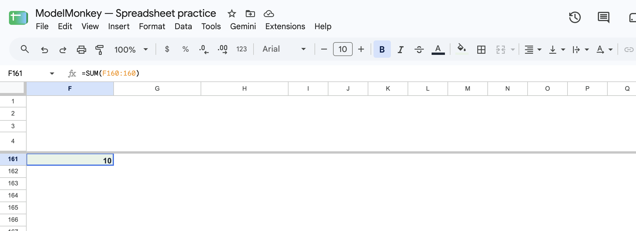
Native Google Sheets accepts this open-ended row range; the Excel download uses F160:H160.
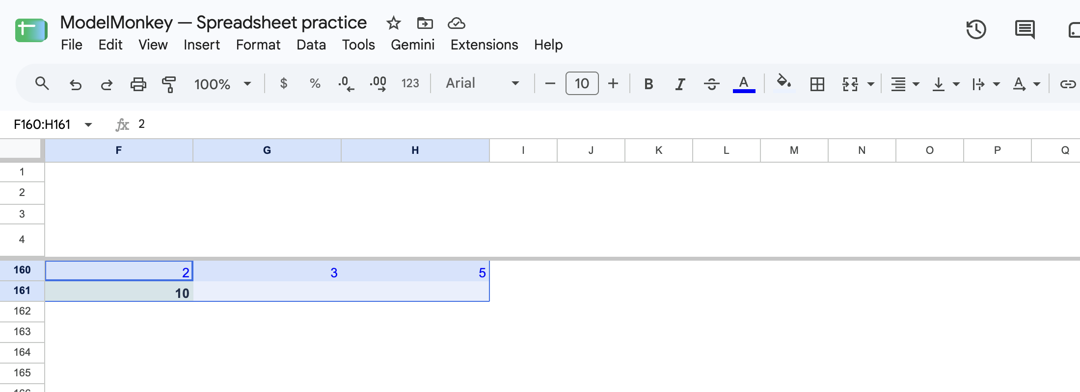
The native Google Sheets row range starts at F160 and extends to the final column in row 160.
Be sure to keep the formula outside row 160. If you place it in an included cell, such as I160, the formula refers to itself and creates a circular reference.
How to read the Google Sheets range F160:160
Each of these references covers a different area:
- F160 identifies one cell.
- F160:H160 covers columns F through H on row 160.
- 160:160 covers the entire row.
- F160:160 begins at column F and covers the rest of row 160.
Google’s A1 notation documentation explains cell, row, column, and sheet-qualified references. Separately, the recorded spreadsheet execution confirms that native Google Sheets accepted F160:160 in this example.
Since the range begins at F, it excludes columns A through E. It also includes cells after H, whether they’re populated now or later.
F160:160 versus the bounded range F160:H160
| Formula | Cells included | Appropriate use |
|---|---|---|
| =SUM(F160:160) | F160 through the final column of row 160 | Values added farther right should enter the total |
| =SUM(F160:H160) | Only F160 through H160 | The calculation must stop at a defined column |
For the supplied inputs, both formulas have an expected result of 10 when cells to the right make no net numeric contribution.
Now suppose you enter 4 in I160 later:
- The open-ended formula would include I160, producing 14.
- The bounded formula would continue to include only F160:H160, producing 10.
Those results follow from the range definitions. Only the original 2 + 3 + 5 example was part of the recorded execution.
In an FP&A schedule with a fixed reporting horizon, a bounded range makes the endpoint explicit and reduces the risk of including an unrelated value added farther to the right. The open-ended form is more appropriate when new periods or categories added to the right should enter the calculation automatically.
Blank cells after H160 don’t affect SUM. SUM also ignores text in the range but includes numeric values.
For formulas that return results across multiple cells instead of a single total, see ARRAYFORMULA Function in Google Sheets.