
Recalculation only reevaluates existing formulas. It won’t repair an incorrect formula, convert text to a number, or confirm that an external data source is current.
Check whether the result is actually stale
Before forcing recalculation, confirm that:
- The result cell contains a formula rather than a pasted value.
- Every required input is numeric and free of formula errors.
- You can calculate the expected result independently.
Displayed rounding can also make a result look stale. Check the underlying value in the formula bar before changing the model.
For example, a quote with quantity 10, unit price 25, a 10% discount, and 8% tax should produce:
- Subtotal:
10 × 25 = 250 - Discount:
250 × 0.1 = 25 - Net amount:
250 - 25 = 225 - Tax:
225 × 0.08 = 18 - Total:
225 + 18 = 243
If the sheet shows a different result, inspect the inputs and formulas before assuming recalculation is the problem.
Force recalculation by changing a referenced cell
For an isolated formula:
- Record the current value of an input referenced by the formula.
- Replace it with a different valid value.
- Press Enter.
- Restore the original value if needed and press Enter again.
- Compare the result with an independently calculated expectation.
Entering the same value again doesn’t create a reproducible dependency change. Temporarily changing a financial input in a larger model also creates control risk. A dedicated recalculation key lets you trigger the dependency without changing the calculated amount.
Reproduce a zero-impact recalculation check
Use the synthetic Google Sheets Recalculation Check example:
Open the Recalc Check tab and review Recalc Check!A1:C16.
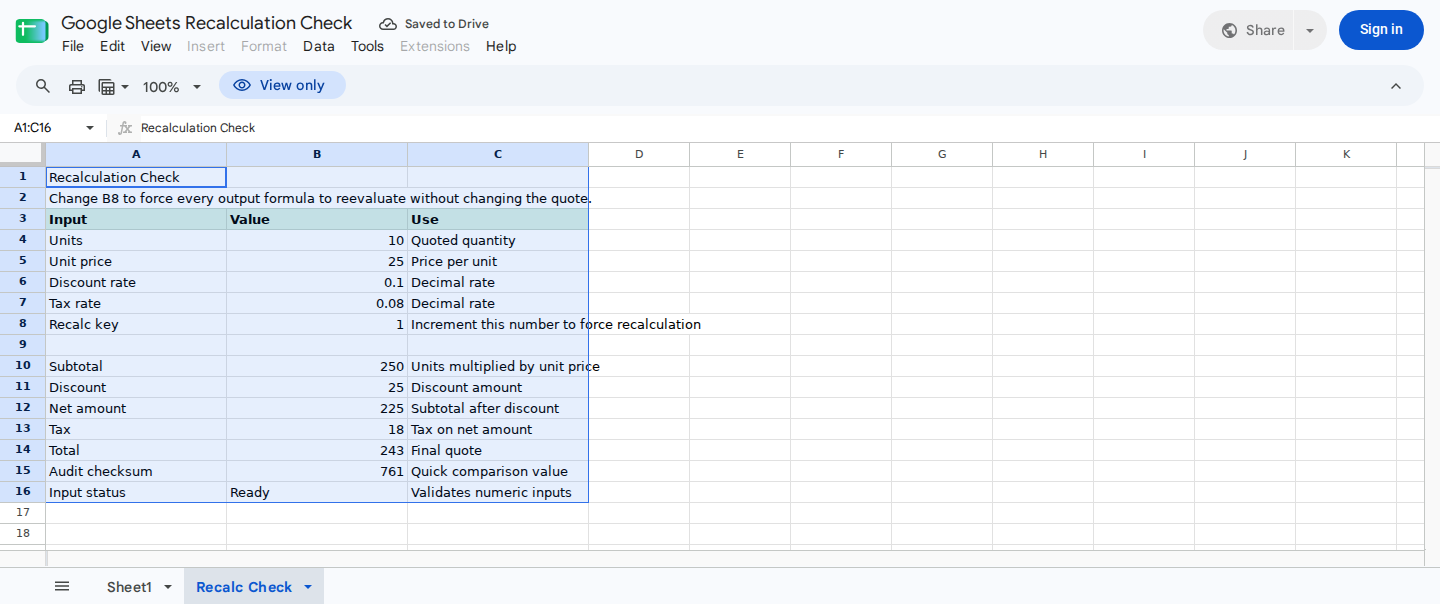
Change cell B8 to make every output formula reevaluate without affecting the quote values.
Follow these steps:
- Enter the quoted quantity in
Recalc Check!B4and the unit price inRecalc Check!B5. - Enter decimal discount and tax rates in
Recalc Check!B6andRecalc Check!B7. For example, enter0.1for 10%. - Review the calculated subtotal, discount, net amount, tax, and total in
Recalc Check!B10:B14. - If the results appear stale, replace
Recalc Check!B8with a different finite number and press Enter. BecauseRecalc Check!B10:B15referenceB8as a zero-impact dependency, they will reevaluate without changing the quote. - Confirm
Recalc Check!B16readsReady. If it readsCheck inputs, correct nonnumeric values inRecalc Check!B4:B8. - Use
Recalc Check!B15as a compact audit value when comparing results before and after recalculation. Do not editRecalc Check!B10:B16.
Formulas behind the check
Each output formula first checks B16, then includes 0*$B$8. Changing B8 updates a referenced dependency, but the added value remains zero.
| Cell | Meaning | Formula |
|---|---|---|
B10 | Subtotal | =IF($B$16="Ready",$B$4*$B$5+0*$B$8,NA()) |
B11 | Discount | =IF($B$16="Ready",B10*$B$6+0*$B$8,NA()) |
B12 | Net amount | =IF($B$16="Ready",B10-B11+0*$B$8,NA()) |
B13 | Tax | =IF($B$16="Ready",B12*$B$7+0*$B$8,NA()) |
B14 | Total | =IF($B$16="Ready",B12+B13+0*$B$8,NA()) |
B15 | Audit checksum | =IF($B$16="Ready",SUM(B10:B14)+0*$B$8,NA()) |
B16 | Input status | =IF(AND(ISNUMBER(B4),ISNUMBER(B5),ISNUMBER(B6),ISNUMBER(B7),ISNUMBER(B8)),"Ready","Check inputs") |
These formulas use commas as argument separators. Some Google Sheets locales require semicolons instead.
The checksum isn’t a financial statement total. It’s a compact control value equal to the sum of B10:B14.
Check the recorded results
The recorded Google Sheets tests cover the following independent cases. Reset all 5 inputs for each case rather than carrying values forward.
| Case | Inputs: B4, B5, B6, B7, B8 | Expected B10:B15 | B16 |
|---|---|---|---|
| Baseline | 10, 25, 0.1, 0.08, 1 | 250, 25, 225, 18, 243, 761 | Ready |
| Recalculation key changed | 10, 25, 0.1, 0.08, 2 | 250, 25, 225, 18, 243, 761 | Ready |
| Quantity changed | 12, 25, 0.1, 0.08, 3 | 300, 30, 270, 21.6, 291.6, 913.2 | Ready |
| Zero quantity | 0, 25, 0.1, 0.08, 4 | 0, 0, 0, 0, 0, 0 | Ready |
The first two cases confirm that changing B8 has no numeric effect on the quote. However, they don’t prove by themselves that reevaluation occurred. A cached result would produce the same visible values and checksum. Proving that calculation occurred would require an execution trace or another observable recalculation indicator.
The quantity-change case provides an independent control. A quantity of 12 produces a subtotal of 300 and a total of 291.6. Meanwhile, the zero-quantity case confirms that numeric zero is treated as a valid input rather than a missing value.
Set Google Sheets calculation options
Google Sheets provides workbook-level calculation settings. Under Google’s documented calculation settings, open:
- File
- Settings
- Calculation
- Recalculation
Choose the appropriate timing for the workbook, then save the setting. Options include recalculating when values change and at time-based intervals.
Time-based calculation can help with formulas based on dates, times, or random values. Still, it doesn’t prove that an external service has supplied current data.
Use iterative calculation only for intentional circular logic
The same settings area contains iterative-calculation controls. These controls repeat circular calculations until an iteration limit or convergence threshold is reached.
Don’t enable iterative calculation merely because an ordinary formula appears stale. First, determine whether the model intentionally contains circular logic. If it doesn’t, trace and remove the circular reference.
For an intentional circular model, document:
- Why the circular relationship is necessary
- The maximum iteration count
- The convergence threshold
- The control used to identify a failure to converge
Troubleshoot results that still appear stale
Except for the 4 recorded cases above, the checks in this section are recommended diagnostics rather than supplied execution tests.
Nonnumeric or blank inputs
B16 checks whether every cell in B4:B8 is numeric. Text, blanks, and whitespace-only text produce Check inputs. The output formulas then return #N/A instead of silently treating malformed input as zero.
In a separate test copy, place text, a blank, and whitespace-only text into each input cell one at a time. Confirm that B16 changes to Check inputs.
Rates outside the intended range
The status formula checks the data type, not whether a value is reasonable for the model. A discount rate of -0.1 is numeric even if negative discounts are invalid for the model.
If rates must remain between 0% and 100%, apply a validation rule to B6:B7:
- Select
B6:B7and open Data > Data validation. - Add a rule whose criterion is Number: between
0and1. - Under the invalid-data behavior, select Reject the input rather than Show a warning.
- Test direct entries of
0and1, followed by values below0and above1.
Only a rule configured to reject input supports the expectation that those direct entries will be rejected. Don’t assume the rule validates every imported or pasted data path. Keep B16 and other model controls in place.
Circular references
A circular-reference warning indicates a formula-design problem, not simply a stale result. Trace the cells that feed each other, and use iterative calculation only when the relationship is intentional and controlled.
Volatile formulas
Functions that change with time or calculation can produce different outputs across reviews. Check the workbook’s calculation setting. Where practical, isolate volatile formulas from core forecast logic.
External-data delays
Changing B8 targets formulas that reference it. It doesn’t guarantee that an import, custom function, or connected data source has returned fresh data.
Check source permissions, displayed errors, timestamps where available, and the external function’s refresh behavior. For the distinction between calculation and collaborative updates, see Does Google Sheets Update in Real Time?.
Incorrect formulas or pasted values
Recalculation can’t correct a wrong reference or restore a formula that was overwritten with a value. Compare each result cell with the intended calculation chain, then reconcile the outputs with an independent control.
Inspect recalculation issues with ModelMonkey
ModelMonkey can inspect the active Google Sheets context, read ranges and formula errors, analyze sheet content, and help change spreadsheet values or formulas. When the workflow presents a preview, review the proposed changes before proceeding. Check each diagnosis and edit rather than assuming it’s correct.
For this workbook, open the ModelMonkey sidebar with Recalc Check!B4:B16 selected and enter:
Inspect Recalc Check!B4:B16. Identify nonnumeric inputs or formula errors, verify the relationships from subtotal through total, and explain any proposed change before editing the output formulas.
After any change, confirm that B16 reads Ready, then reconcile B10:B15 with the expected calculations above.