
The search phrase “cara menghapus cell kosong di spreadsheet” means “how to delete empty cells in a spreadsheet.” In a finance table, however, you need to distinguish between an empty cell, a partially completed record, and a wholly empty row.
Use the verified transaction example
Copy this Google Sheets template or download the Excel file. The synthetic workbook is titled Spreadsheet formula and cleanup practice.
Use the Google Sheets copy for the native QUERY example. The XLSX file provides the source data, guidance, and portable formulas such as SUM(F160:H160), but it doesn’t contain native Google Sheets QUERY output.
Start with Transactions!A1:F13:
| Column | Meaning |
|---|---|
| A | Date |
| B | Category |
| C | Description |
| D | Amount (USD) |
| E | Paid |
| F | Owner |
Rows 5 and 10 are wholly blank. By contrast, rows 8, 9, 11, and 12 are partial records that must remain. For example, row 8 has no Category, but it still contains the description Uncategorized receipt and an amount of USD 14.
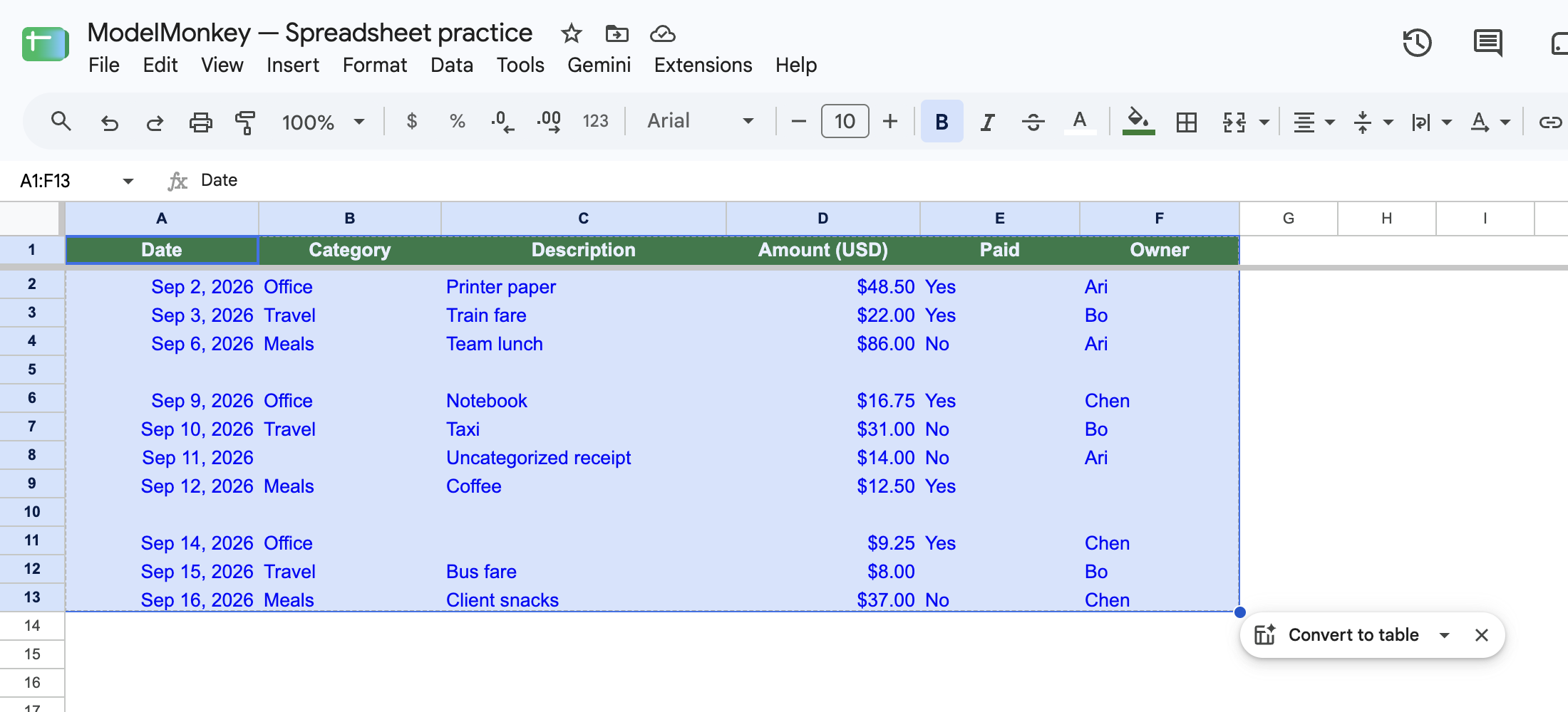
Method 1: Flag wholly blank rows with a helper column
In G1, enter Status. Then enter this formula in G2:
=IF(COUNTA(A2:F2)=0,"DELETE CANDIDATE","KEEP")
Fill the formula through G13.
You should get the following result:
- Original rows 5 and 10:
DELETE CANDIDATE - All 10 transaction rows:
KEEP
Because the formula checks all six fields, a blank Category or Owner alone won’t mark a transaction for deletion.
COUNTA treats numeric zero, whitespace, and a formula returning "" as values, so rows containing them remain. Only a truly empty row returns zero. Google documents this behavior in its COUNTA function guidance.
You can identify incomplete records separately. Enter this formula in H2 and fill it down:
=IF(AND(COUNTA(A2:F2)>0,COUNTBLANK(A2:F2)>0),"REVIEW","COMPLETE OR EMPTY")
Now perform two separate filter checks:
- Filter column G to
DELETE CANDIDATEand review the wholly empty rows. - Clear the filter condition on G.
- Filter column H to
REVIEWand inspect the partial records.
Don’t leave both conditions active. If you do, no rows will appear because a wholly empty row receives COMPLETE OR EMPTY in column H. Separate filter views are another option. Google explains the available filter and filter-view controls.
Method 2: Delete the verified blank rows
Before making destructive changes, duplicate the Transactions tab. In the duplicate:
- Select the entire row 10 and choose Delete row.
- Select the entire row 5 and choose Delete row.
Work from bottom to top so deleting row 10 doesn’t affect the position of row 5. Google’s documentation distinguishes deleting rows from deleting cells and shifting adjacent data.
The recorded Google Sheets execution produced a cleaned range of A1:F11, containing one header and 10 transactions. It also preserved the partial receipt at:
C7:Uncategorized receiptD7:14
Check those cells after deletion to confirm that the data remains aligned.
Method 3: Create a non-destructive QUERY view
If every valid transaction must have a Date, enter this formula in Practice!A18:
=QUERY(Transactions!A1:F13,"select * where A is not null",1)
It follows Google’s documented QUERY(data, query, [headers]) syntax.
The expected output is Practice!A18:F28, with one header followed by 10 dated records in their original order. In the recorded execution, all four partial records remained, including the uncategorized USD 14 receipt.
This approach does have a limitation: it excludes any valid record with a blank Date. Confirm that column A is a mandatory key before using it. If it isn’t, rely on the whole-row helper instead.
Some spreadsheet locales require semicolons rather than commas between formula arguments. For more examples, see How to Use QUERY in Google Sheets for Finance.
Reconcile the cleaned result
Before replacing the source, check more than the visible gaps:
| Control | Expected result |
|---|---|
| Surviving transaction records | 10 |
| Wholly blank rows removed | 2 |
| Partial records retained | 4 |
| Amount total before cleanup | USD 285.00 |
| Amount total after cleanup | USD 285.00 |
| Formula errors introduced | 0 |
You can reproduce the amount control from the 10 source amounts:
48.50 + 22.00 + 86.00 + 16.75 + 31.00
+ 14.00 + 12.50 + 9.25 + 8.00 + 37.00
= 285.00
Matching totals alone aren’t enough. Also confirm that the surviving six-field records remain in the same order and that descriptions, amounts, payment statuses, and owners are still aligned.
This whole-record method was also executed on 10,000 data slots. It removed 500 empty slots while retaining 9,500 records, including 2,000 partial records. The surviving field values and order matched, the amount total remained USD 116,294.75, and no formula errors were found.
Use ModelMonkey for the same cleanup job
ModelMonkey can inspect and organize spreadsheet ranges in Google Sheets or Excel using natural-language instructions. For this example, you could enter:
On a duplicate of Transactions, inspect A1:F13. Identify only rows where all six cells are empty, preserve partial records, delete whole rows, and report the surviving record count and Amount total. Do not modify the source tab.
Where the workflow presents a preview, review the proposed row changes before proceeding. Afterward, verify the result independently. You should have 10 records, a USD 285.00 total, and Uncategorized receipt still paired with USD 14.