
You can also use a keyboard shortcut. Google documents Ctrl + Shift + V for Windows and ChromeOS and ⌘ + Shift + V for Mac as Paste values only shortcuts.
Before converting finance calculations, preserve the original formulas in a duplicate sheet or separate live-output cells. Once a formula becomes a fixed value, it won't change when its source data changes.
Remove a formula while keeping its value
Follow these steps to replace a formula with its current result:
- Duplicate the sheet or preserve the formula in another cell.
- Select and copy the formula cell or range.
- Without changing the selection, choose Edit → Paste special → Values only.
- Select a converted cell and inspect the formula bar.
The displayed result should stay the same. In the formula bar, you should now see a number, date, or text instead of an expression beginning with =.
In the supplied demonstration workbook, Practice!B15 contains:
=SUMIFS(Transactions!$D$2:$D$13,Transactions!$B$2:$B$13,"Office")
The formula uses Transactions!B2:B13 for categories and Transactions!D2:D13 for amounts. Its three Office records total:
48.5 + 16.75 + 9.25 = 74.5 USD
If you copy Practice!B15 and paste values only back into the same cell, it will still display 74.5, but the formula will be gone. Only perform that test in a disposable copy.
For a safer setup, use the arrangement shown in Practice!B15:C15. Cell B15 retains the formula, while C15 contains the fixed numeric value 74.5.
Some spreadsheet locales use semicolons instead of commas between formula arguments. That doesn't change the values-only procedure.
Freeze a month-end output without deleting the formulas
For an approved forecast or month-end reporting output, keep the live calculations and place the frozen results in separate snapshot cells. This arrangement preserves the formulas for review and prevents the approved output from changing automatically.
Use the synthetic Spreadsheet formula and cleanup practice workbook:
Both files contain the Snapshot tab. Starting from the original baseline:
- Copy
Practice!B15and paste Values only intoSnapshot!C5. - Copy
Practice!B16, which contains=SUM(Transactions!D2:D13), and paste Values only intoSnapshot!C6. - Retain the original formulas in
Practice!B15:B16. - Confirm that
Snapshot!B5:B6remain linked to the live outputs. - Confirm that
Snapshot!D5:D6calculate live minus frozen.
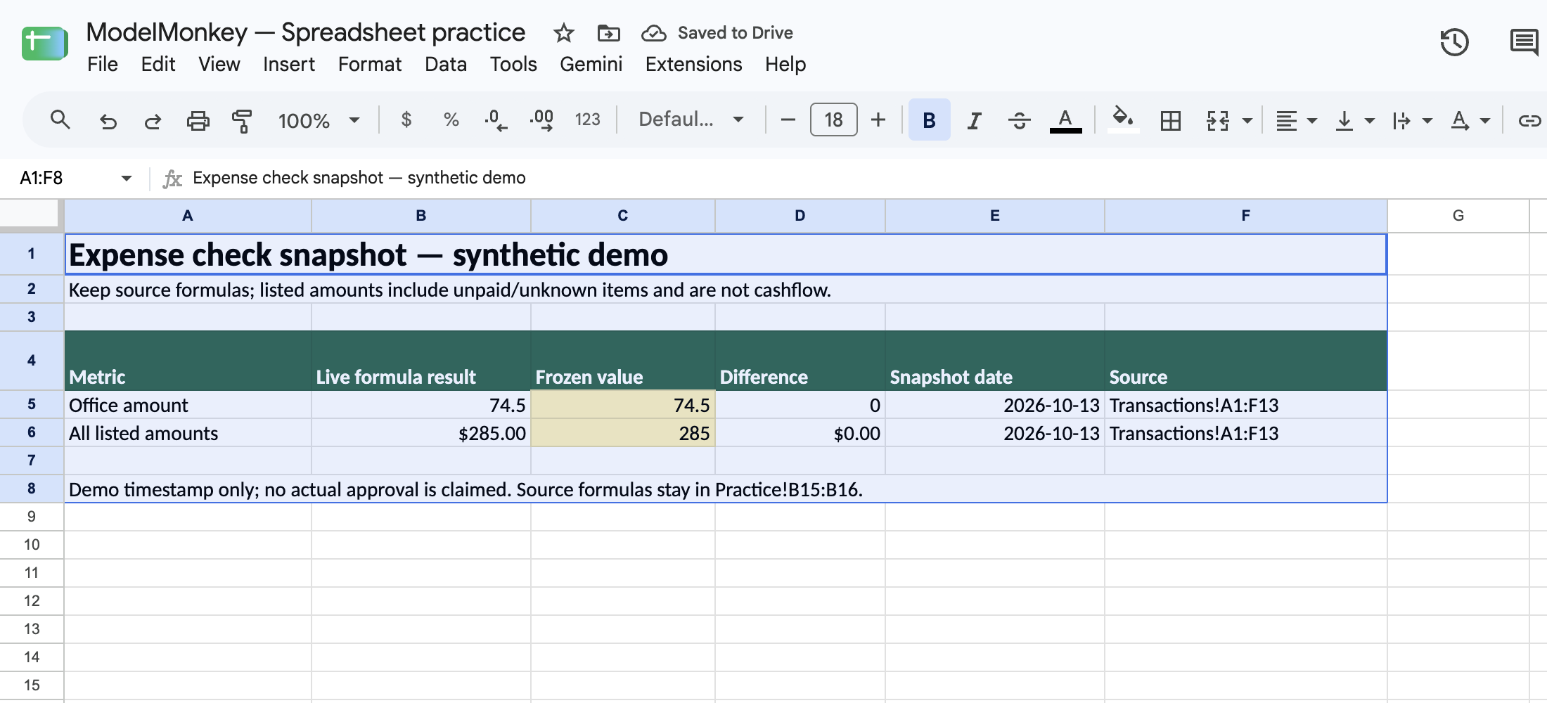
Formula outputs are retained; fixed values carry a date and source note.
The verified baseline in Snapshot!A1:F8 is:
| Cell | Control purpose | Expected result |
|---|---|---|
Snapshot!B5 | Live Office total | 74.5 |
Snapshot!C5 | Frozen Office value | 74.5 |
Snapshot!D5 | Live minus frozen | 0 |
Snapshot!B6 | Live total of listed amounts | 285 |
Snapshot!C6 | Frozen total | 285 |
Snapshot!D6 | Live minus frozen | 0 |
The 285 control consists of:
48.5 + 22 + 86 + 16.75 + 31 + 14 + 12.5 + 9.25 + 8 + 37
= 285 USD
This figure includes unpaid records and records with a missing category or payment status. It isn't a cash-flow total.
For a repeatable month-end control, record these fields beside the frozen values:
| Control field | Entry |
|---|---|
| Reporting period | Approved forecast or reporting period |
| Source | Transactions!A1:F13 |
| Demo snapshot date | 2026-10-13 |
| Prepared by | Snapshot owner |
| Reviewer/sign-off | Reviewer name, review date, and status |
In this demonstration, the reporting-period field is metadata. Neither formula filters the Date column, so the frozen values cover every listed amount in Transactions!A1:F13.
For an actual period-specific forecast, use a formula or source range that applies the required date boundary.
Reconcile live and frozen values
To confirm that the snapshot no longer recalculates, change Transactions!D2 from 48.5 to 49.5 in a copy of the workbook.
The recorded Google Sheets execution produced:
| Control | Baseline | After change |
|---|---|---|
Live Office total, B5 | 74.5 | 75.5 |
Frozen Office value, C5 | 74.5 | 74.5 |
Difference, D5 | 0 | 1 |
Live overall total, B6 | 285 | 286 |
Frozen overall value, C6 | 285 | 285 |
Difference, D6 | 0 | 1 |
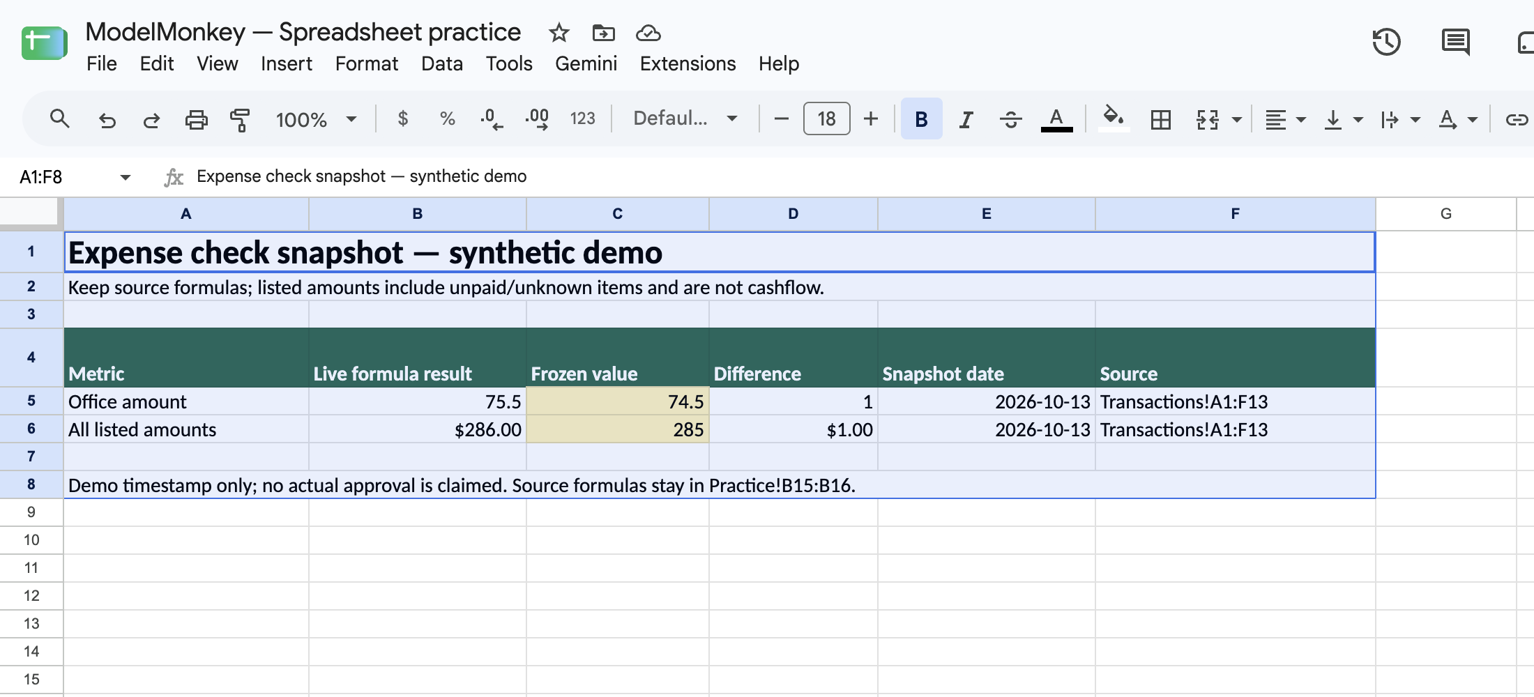
Source amount increased by one; frozen values remain unchanged. Source restored after testing.
Next, restore Transactions!D2 to 48.5. The live totals should return to 74.5 and 285, and both differences should return to 0.
A nonzero difference means the live calculation has changed since the snapshot was created. Before sign-off, review the source change and confirm the frozen period and source. Then decide whether to keep the historical snapshot fixed or refresh it.