
Build a 5-Year Projection in Google Sheets
Build and verify a five-year Google Sheets forecast with revenue, expenses, cash, scenarios, formulas, and reconciliation checks.
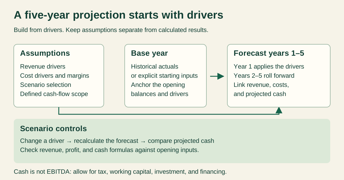
Download the editable five-year projection workbook below and import it into Google Sheets, or follow the cell-by-cell instructions to build your own. The completed workbook forecasts FY2027 through FY2031, switches among 3 scenarios, and includes visible reconciliation checks for revenue, EBITDA, and cash.
The example uses annual calendar periods and USD. It covers revenue, COGS, gross profit, operating expenses, EBITDA, net cash change, and ending cash.
To keep the example reproducible, net cash change equals EBITDA. Taxes, working capital, capital expenditure, financing, depreciation, and balance-sheet forecasting are excluded.
What You'll Need
- A blank Google Sheets workbook
- FY2026 revenue, operating expenses, and closing cash inputs
- Permission to edit the workbook
- A decision to use calendar years from January 1 through December 31
Step-by-Step Guide
Define what the projection template must include
Download the editable projection workbook (.xlsx). It contains the two tabs, formulas, three scenarios, reconciliation checks, and illustrative values used in this guide. No sign-up is required.
To use it in Google Sheets, open a new spreadsheet, choose File > Import > Upload, select the downloaded workbook, and import it as a new spreadsheet. Keep the original download as a reference copy. Google documents the supported import options in its Excel-to-Sheets guide.
Start with the Base case. Confirm FY2031 EBITDA of $202,371.06, ending cash of $838,262.18, and all 15 check cells showing OK before changing the editable input cells. Then select Optimistic and Conservative in Assumptions!B2 and compare the scenario totals shown below. If imported formulas or dates differ, stop and inspect them before using the output.
This is a compact operating projection, not an investor-ready three-statement forecast. Its cash row deliberately equals EBITDA before excluded cash items; do not use that row as a real cash-flow forecast until those components are modeled.
A five-year financial projection template should separate inputs from calculations and clearly define its forecast periods. Whether you use an existing template or build one, check that it has:
- A dedicated assumptions area
- Actual date values for each forecast year
- Revenue, COGS, gross profit, operating expenses, and EBITDA
- A cash roll-forward
- Base, optimistic, and conservative scenarios
- Formulas that can be inspected
- Checks tying subtotals and cash movements together
Don’t select a template solely because it has polished formatting. First, determine whether its formulas, units, period definitions, and scenario mechanics are visible.
For this example, create exactly 2 tabs:
AssumptionsProjection
Enter the opening assumptions and scenario table
On the Assumptions tab, enter these labels and illustrative values:
| Cell | Entry | Meaning |
|---|---|---|
| A2 | Selected scenario | Input label |
| B2 | Base | Active scenario |
| A4 | FY2026 revenue | Input label |
| B4 | 500000 | FY2026 revenue in USD |
| A5 | FY2026 operating expenses | Input label |
| B5 | 220000 | FY2026 operating expenses in USD |
| A6 | Opening cash at 12/31/2026 | Input label |
| B6 | 100000 | Cash immediately before FY2027 |
| A8 | Selected revenue growth | Calculated label |
| A9 | Selected OpEx growth | Calculated label |
| A10 | Selected gross margin | Calculated label |
Next, enter the scenario table in A13:D16:
| Scenario | Revenue growth | OpEx growth | Gross margin |
|---|---|---|---|
| Base | 10% | 5% | 60% |
| Optimistic | 15% | 7% | 63% |
| Conservative | 3% | 4% | 55% |
Revenue and OpEx growth can legitimately exceed 100%; 150% growth multiplies the prior amount by 2.5. This worked template deliberately limits growth to -100% through 100% as an illustrative input policy, not as a mathematical bound on growth. If your forecast needs a higher growth rate, change the upper limit consistently in data validation, the selected-rate formulas in Assumptions!B8:B9, and the Projection growth guards, then rerun the boundary and reconciliation checks. The 0% through 100% gross-margin limit is a different constraint and remains in place.
The scenario names must use exactly the capitalization shown.
Apply these data-validation rules through Data > Data validation > Add rule:
B2: dropdown containingBase,Optimistic, andConservative; reject invalid entries.B4:B6: number greater than or equal to0.B14:C16: number between-100%and100%.D14:D16: number between0%and100%.
Format B4:B6 as USD and B14:D16 as percentages. Also format Assumptions!B8:B10 as percentages; these calculated cells do not automatically inherit the scenario-table format. The formulas below also check data types and permitted ranges, keeping invalid assumptions visible when the source cells don’t contain valid numbers.
Connect the selected scenario to the assumptions
The selected-rate formulas must validate both the scenario name and its corresponding rate cell. This prevents a blank scenario-rate cell from being treated as 0%.
Enter this formula in Assumptions!B8:
=IF(AND(SUMPRODUCT(--EXACT($B$2,$A$14:$A$16))=1,SUMPRODUCT(--EXACT($B$2,$A$14:$A$16),--ISNUMBER($B$14:$B$16),--($B$14:$B$16>=-100%),--($B$14:$B$16<=100%))=1),INDEX($B$14:$B$16,MATCH(TRUE,EXACT($B$2,$A$14:$A$16),0)),NA())
With B2 set to Base, the expected result is 10%.
Enter this formula in Assumptions!B9:
=IF(AND(SUMPRODUCT(--EXACT($B$2,$A$14:$A$16))=1,SUMPRODUCT(--EXACT($B$2,$A$14:$A$16),--ISNUMBER($C$14:$C$16),--($C$14:$C$16>=-100%),--($C$14:$C$16<=100%))=1),INDEX($C$14:$C$16,MATCH(TRUE,EXACT($B$2,$A$14:$A$16),0)),NA())
The expected Base result is 5%.
Enter this formula in Assumptions!B10:
=IF(AND(SUMPRODUCT(--EXACT($B$2,$A$14:$A$16))=1,SUMPRODUCT(--EXACT($B$2,$A$14:$A$16),--ISNUMBER($D$14:$D$16),--($D$14:$D$16>=0),--($D$14:$D$16<=100%))=1),INDEX($D$14:$D$16,MATCH(TRUE,EXACT($B$2,$A$14:$A$16),0)),NA())
The expected Base result is 60%.
Together, these formulas require exactly one case-sensitive scenario match and a numeric rate within the applicable bounds. A blank selection, lowercase base, unknown scenario, duplicate exact scenario name, blank rate, text rate, or out-of-range rate returns #N/A.
Set up the five-year projection periods
On the Projection tab, enter:
| Cell | Entry |
|---|---|
| A1 | Metric |
| A3 | Revenue |
| A4 | COGS |
| A5 | Gross profit |
| A6 | Operating expenses |
| A7 | EBITDA |
| A8 | Net cash change |
| A9 | Ending cash |
| A11 | Revenue check |
| A12 | EBITDA check |
| A13 | Cash check |
Then enter actual dates across row 1:
B1: =DATE(2027,12,31)
C1: =DATE(2028,12,31)
D1: =DATE(2029,12,31)
E1: =DATE(2030,12,31)
F1: =DATE(2031,12,31)
Each column covers the inclusive calendar year from January 1 through December 31. Apply the custom number format "FY"yyyy so the cells display as FY2027 through FY2031 while preserving the underlying date values.
Before moving on, confirm that there are no skipped or duplicate years and that opening cash in Assumptions!B6 is measured at December 31, 2026.
Build the revenue, cost, and EBITDA forecast
Start by entering the first-year revenue formula in Projection!B3:
=IF(AND(ISNUMBER(Assumptions!$B$4),Assumptions!$B$4>=0,ISNUMBER(Assumptions!$B$8),Assumptions!$B$8>=-100%,Assumptions!$B$8<=100%),Assumptions!$B$4*(1+Assumptions!$B$8),NA())
With FY2026 revenue of 500000 and Base growth of 10%, the expected result is:
500000 × 1.10 = 550000
Enter this formula in Projection!C3 and copy it through F3:
=IF(AND(ISNUMBER(B3),B3>=0,ISNUMBER(Assumptions!$B$8),Assumptions!$B$8>=-100%,Assumptions!$B$8<=100%),B3*(1+Assumptions!$B$8),NA())
Next, enter the COGS formula in Projection!B4 and copy it through F4:
=IF(AND(ISNUMBER(B3),B3>=0,ISNUMBER(Assumptions!$B$10),Assumptions!$B$10>=0,Assumptions!$B$10<=100%),B3*(1-Assumptions!$B$10),NA())
For FY2027, expected COGS is:
550000 × (1 - 60%) = 220000
Enter the gross-profit formula in Projection!B5 and copy it through F5:
=IF(AND(ISNUMBER(B3),ISNUMBER(B4)),B3-B4,NA())
Expected FY2027 gross profit is:
550000 - 220000 = 330000
Now enter the first-year operating-expense formula in Projection!B6:
=IF(AND(ISNUMBER(Assumptions!$B$5),Assumptions!$B$5>=0,ISNUMBER(Assumptions!$B$9),Assumptions!$B$9>=-100%,Assumptions!$B$9<=100%),Assumptions!$B$5*(1+Assumptions!$B$9),NA())
Expected FY2027 operating expenses are:
220000 × 1.05 = 231000
Enter this formula in Projection!C6 and copy it through F6:
=IF(AND(ISNUMBER(B6),B6>=0,ISNUMBER(Assumptions!$B$9),Assumptions!$B$9>=-100%,Assumptions!$B$9<=100%),B6*(1+Assumptions!$B$9),NA())
Finally, enter the EBITDA formula in Projection!B7 and copy it through F7:
=IF(AND(ISNUMBER(B5),ISNUMBER(B6)),B5-B6,NA())
Expected FY2027 EBITDA is:
330000 - 231000 = 99000
Negative EBITDA is allowed and should remain visible. It’s a forecast result, not an invalid input.
Complete the simplified cash roll-forward
In this limited example, EBITDA equals net cash change. Enter this formula in Projection!B8 and copy it through F8:
=IF(ISNUMBER(B7),B7,NA())
For the first year, enter the ending-cash formula in Projection!B9:
=IF(AND(ISNUMBER(Assumptions!$B$6),Assumptions!$B$6>=0,ISNUMBER(B8)),Assumptions!$B$6+B8,NA())
Expected FY2027 ending cash is:
100000 + 99000 = 199000
Enter this formula in Projection!C9 and copy it through F9:
=IF(AND(ISNUMBER(B9),ISNUMBER(C8)),B9+C8,NA())
For FY2028, the expected calculation is:
199000 + 120450 = 319450
A negative cash change can produce negative ending cash. Keep that result visible for review instead of converting it to zero.
Format B3:F9 as USD with 2 decimal places. The formulas retain their underlying precision even when fewer decimals appear.
Verify the Base projection and compare scenarios
With Assumptions!B2 set to Base, the exact expected values before display rounding are:
| Metric | FY2027 | FY2028 | FY2029 | FY2030 | FY2031 |
|---|---|---|---|---|---|
| Revenue | 550000 | 605000 | 665500 | 732050 | 805255 |
| COGS | 220000 | 242000 | 266200 | 292820 | 322102 |
| Gross profit | 330000 | 363000 | 399300 | 439230 | 483153 |
| Operating expenses | 231000 | 242550 | 254677.5 | 267411.375 | 280781.94375 |
| EBITDA | 99000 | 120450 | 144622.5 | 171818.625 | 202371.05625 |
| Net cash change | 99000 | 120450 | 144622.5 | 171818.625 | 202371.05625 |
| Ending cash | 199000 | 319450 | 464072.5 | 635891.125 | 838262.18125 |
With 2-decimal formatting, FY2031 EBITDA should display as $202,371.06, and ending cash should display as $838,262.18.
Next, change Assumptions!B2 to Optimistic. The expected FY2027 results are:
| Metric | Expected FY2027 result |
|---|---|
| Revenue | 575000 |
| COGS | 212750 |
| Gross profit | 362250 |
| Operating expenses | 235400 |
| EBITDA | 126850 |
| Net cash change | 126850 |
| Ending cash | 226850 |
Then change B2 to Conservative. The expected FY2027 results are:
| Metric | Expected FY2027 result |
|---|---|
| Revenue | 515000 |
| COGS | 231750 |
| Gross profit | 283250 |
| Operating expenses | 228800 |
| EBITDA | 54450 |
| Net cash change | 54450 |
| Ending cash | 154450 |
Only the selected rates and their dependent projection cells should change. The original scenario-table inputs should remain fixed.
Add reconciliation checks and test the model
Add formula-based checks so broken identities are visible in the workbook.
Enter this revenue check in Projection!B11 and copy it through F11:
=IF(AND(ISNUMBER(B3),ISNUMBER(B4),ISNUMBER(B5)),IF(ROUND(B3-B4-B5,2)=0,"OK","CHECK"),"CHECK")
Enter this EBITDA check in Projection!B12 and copy it through F12:
=IF(AND(ISNUMBER(B5),ISNUMBER(B6),ISNUMBER(B7)),IF(ROUND(B7-(B5-B6),2)=0,"OK","CHECK"),"CHECK")
For FY2027, enter the cash check in Projection!B13:
=IF(AND(ISNUMBER(Assumptions!$B$6),ISNUMBER(B8),ISNUMBER(B9)),IF(ROUND(B9-(Assumptions!$B$6+B8),2)=0,"OK","CHECK"),"CHECK")
Enter this formula in Projection!C13 and copy it through F13:
=IF(AND(ISNUMBER(B9),ISNUMBER(C8),ISNUMBER(C9)),IF(ROUND(C9-(B9+C8),2)=0,"OK","CHECK"),"CHECK")
These checks test the following identities to the nearest cent:
Revenue = COGS + Gross profit
EBITDA = Gross profit - Operating expenses
Ending cash = prior cash + Net cash change
For FY2027, prior cash is Assumptions!B6. From FY2028 onward, it’s the preceding year’s ending cash. With the supplied Base, Optimistic, or Conservative assumptions, every cell in Projection!B11:F13 should display OK.
The downloadable Excel workbook was recalculated in LibreOffice 26.8 across 28 scenario, invalid-input, and boundary cases. Base, Optimistic, and Conservative produced the stated totals, with all 15 checks showing OK. Invalid assumptions produced visible #N/A errors and CHECK controls. These tests did not include a Google Sheets import. After importing or customizing, rerun the controls below in your spreadsheet application; a successful desktop recalculation does not establish that an imported copy behaves identically:
| Check | Action | Expected result |
|---|---|---|
| Base case | Select exact Base | Every projection value matches the five-year Base table; B11:F13 displays OK |
| Scenario case | Select Optimistic, then Conservative | FY2027 values match the scenario tables; B11:F13 remains OK |
| Case sensitivity | In an unvalidated copy, enter base | Assumptions!B8:B10 shows #N/A; projections show #N/A; checks show CHECK |
| No match | In an unvalidated copy, enter Upside or clear B2 | Selected rates and projections show #N/A, not zero |
| Duplicate key | Replace another scenario name with a second exact Base in A14:A16 | B8:B10 shows #N/A because there are 2 exact matches |
| Zero inputs | Set opening revenue and OpEx to numeric 0, leaving cash at 100000 | Revenue through net cash change remain zero; ending cash remains 100000; checks show OK |
| Blank opening revenue | Clear B4 | Revenue and dependent formulas show #N/A |
| Text opening revenue | Enter five hundred thousand in an unvalidated copy | Revenue and dependent formulas show #N/A |
| Other opening inputs | Repeat the blank and text tests for B5 and B6 | Their dependent formulas show #N/A |
| Blank selected rate | Clear B14, C14, or D14 in separate Base-case copies | The corresponding selected rate in B8, B9, or B10 shows #N/A; dependent formulas don’t calculate with 0% |
| Text selected rate | Enter text in B14, C14, or D14 in separate unvalidated copies | The corresponding selected rate and dependent formulas show #N/A |
| Revenue-growth guard | In an unvalidated copy, set selected revenue growth to 150% | B8 and revenue-dependent formulas show #N/A |
| OpEx-growth guard | In an unvalidated copy, set selected OpEx growth to -120% | B9 and operating-expense-dependent formulas show #N/A |
| Gross-margin guard | In separate unvalidated copies, set selected gross margin to 105% and -5% | B10, COGS, and dependent formulas show #N/A |
| Revenue-growth boundary | Set selected revenue growth to -100%, then 100% | -100% makes the next forecast revenue zero; 100% doubles it |
| Gross-margin boundary | Set selected gross margin to 0%, then 100% | At 0%, COGS equals revenue; at 100%, COGS equals zero |
| Date boundary | Inspect B1:F1 | Cells contain December 31 dates for 2027-2031 with no skipped or duplicate year |
| Opening-entry control | Inspect Assumptions!B4:B6 | There is exactly one opening revenue, OpEx, and cash input |
| Arithmetic reconciliation | Inspect Projection!B11:F13 | All 15 check cells display OK when the 3 identities hold |
These controls test arithmetic consistency. They don’t establish that the assumptions are commercially reasonable or that the simplified cash treatment is suitable for a real planning decision.
If you add more opening entries while customizing the workbook, reconcile them manually first. The formulas don’t detect or exclude duplicate opening balances automatically.
Google Sheets locales that use semicolons as formula separators may require replacing each comma in the formulas with a semicolon. Check Google’s locale and calculation settings and function reference when adapting the formulas.
Customize the projection without breaking its controls
Replace the illustrative inputs only after the Base case matches the expected results and every reconciliation cell displays OK.
For a specific business or finance use case:
- Document whether every amount is USD, another currency, units, or a percentage.
- State whether periods are calendar or fiscal years.
- Replace generic growth rates with business-specific drivers only after defining their units.
- Keep scenario inputs separate from projection formulas.
- Preserve the 3 reconciliation checks.
- Extend net cash change only when you’re ready to model the excluded cash-flow components explicitly.
- Retest Base, Optimistic, and Conservative after changing the structure.
If you start from an existing template, map its cells to the same input, calculation, and control categories before relying on its outputs.
Use ModelMonkey to inspect and present the projection
ModelMonkey is an AI assistant for Google Sheets and Excel. In Google Sheets, it can use the active spreadsheet, sheet, and selected-range context to read ranges, inspect formula errors, organize content, assist with formulas, analyze outputs, and create or adjust charts.
For this workbook, select Projection!B3:F13 and ask ModelMonkey:
Inspect this five-year projection for formula errors. Check whether the Revenue, EBITDA, and Cash control rows agree with their underlying formulas in every year. List any discrepancies without changing cells.
Review its findings against the expected results in this guide. AI assistance doesn’t replace checking the workbook’s formulas or business assumptions.
To present the forecast, create a line chart using:
- X-axis:
Projection!B1:F1 - Revenue series:
Projection!B3:F3 - EBITDA series:
Projection!B7:F7 - Ending-cash series:
Projection!B9:F9
You can ask ModelMonkey to help create or adjust this chart. When its workflow presents proposed spreadsheet changes for review, inspect them before proceeding. For more guidance on checking AI-generated formulas, see Google Sheets AI Formula Tools for FP&A.
Wrapping Up
The completed workbook produces a five-year annual projection for FY2027 through FY2031, switches between 3 scenarios, returns visible errors for invalid selected rates, and includes formula-based revenue, EBITDA, and cash checks.
Confirm the supplied Base and scenario results before replacing the illustrative assumptions or expanding the simplified cash treatment.
Frequently Asked Questions
Can I download an Excel workbook for use in Google Sheets?
Yes. Download the editable .xlsx workbook for import into Google Sheets using File > Import > Upload. Google supports Excel imports; this workbook has been recalculated in LibreOffice, but its Google Sheets import has not been tested. It includes the exact two-tab example, scenario inputs, formulas, and reconciliation checks described here. Check the supplied Base totals after import. It is a simplified operating projection, not a full three-statement cash forecast.
How should I evaluate a five-year projection template I find online?
Check whether it separates inputs from formulas, uses real dates, states units, exposes scenario assumptions, and contains formula-based reconciliation controls. Don’t rely on a template until you can trace its outputs back to documented inputs.
Why does the template return #N/A instead of zero?
#N/A makes invalid, missing, duplicated, nonnumeric, or out-of-range assumptions visible. Returning zero could make an incomplete forecast appear valid.
What does CHECK mean in the reconciliation rows?
CHECK means an input isn’t numeric or an identity fails to reconcile to the nearest cent. Trace that column’s formulas and upstream assumptions before relying on its output.
Can I change the model to monthly periods?
Yes, but the formulas and opening-balance logic must be redesigned for 60 monthly columns. Don’t relabel the annual columns as months without changing growth-rate periodicity and cash calculations.
Is EBITDA normally the same as net cash change?
No. That equality is a deliberate simplification for this example. A fuller cash forecast may need taxes, working-capital movements, capital expenditure, financing, and other cash items.
Can I use fiscal years instead of calendar years?
Yes. Replace the dates in Projection!B1:F1 with the correct fiscal year-end dates and document the period covered by each column. Keep five consecutive, nonoverlapping 12-month periods.
What should I do if my formulas require semicolons?
Some Google Sheets locales use semicolons rather than commas between function arguments. Replace the commas used as argument separators with semicolons; don’t alter decimal or percentage values.