
Build a Startup 3-Statement Financial Model
Build and verify a six-month startup model linking revenue, schedules, income statement, cash flow, balance sheet, and funding needs.
This guide shows finance and FP&A analysts how to build an integrated startup financial model in Google Sheets or Excel. The completed six-month model links operating assumptions to the income statement, cash flow statement, and balance sheet. It also includes checks for cash reconciliation and the accounting equation.
The worked example is illustrative and models a SaaS startup from January through June 2027 in USD. It excludes deferred revenue, inventory, dividends, debt covenants, asset retirements, tax-loss carryforwards, valuation, and transaction-level data.
What You'll Need
- Google Sheets or Microsoft Excel
- Familiarity with relative and absolute cell references
- A workbook with these 5 tabs, in this order:
Inputs,Revenue,Schedules,Statements, andChecks - Formulas configured with comma argument separators; replace commas with semicolons if required by your spreadsheet locale
- Rates entered as decimals and displayed as percentages
- Customer counts allowed to be fractional because churn is modeled as an expected value
Step-by-Step Guide
Set up the timeline and startup assumptions
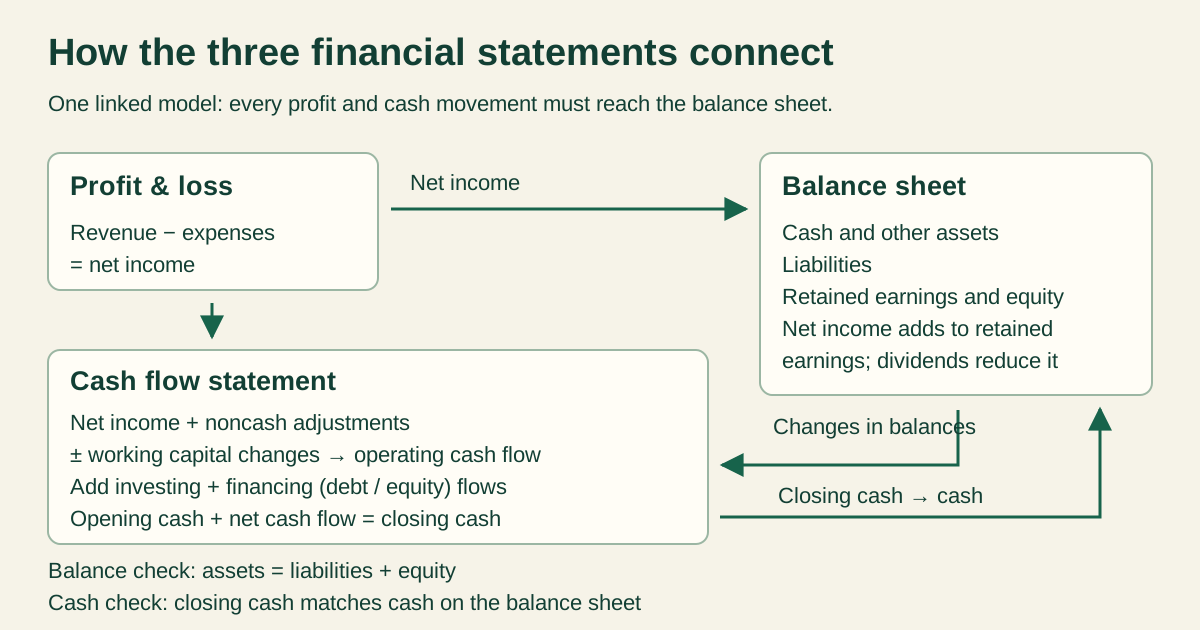
A three-statement model connects three core reports:
- The income statement, which calculates profit or loss over each month
- The cash flow statement, which reconciles beginning cash to ending cash
- The balance sheet, which shows assets, liabilities, and equity at each month-end
Enter these dates in Inputs!B1:G1:
| Cell | Date |
|---|---|
| B1 | 2027-01-31 |
| C1 | 2027-02-28 |
| D1 | 2027-03-31 |
| E1 | 2027-04-30 |
| F1 | 2027-05-31 |
| G1 | 2027-06-30 |
The model must contain exactly these 6 forecast columns. On each of the other 4 tabs, enter =Inputs!B1 in B1 and copy it through G1.
Next, enter the following monthly assumptions on Inputs:
| Row | Assumption | Jan | Feb | Mar | Apr | May | Jun |
|---|---|---|---|---|---|---|---|
| 2 | New customers | 5 | 5 | 5 | 5 | 5 | 5 |
| 3 | Churn rate | 5% | 5% | 5% | 5% | 5% | 5% |
| 4 | Monthly ARPU | 1,000 | 1,000 | 1,000 | 1,000 | 1,000 | 1,000 |
| 5 | Ending headcount | 2 | 2 | 3 | 3 | 3 | 3 |
| 6 | Monthly salary per employee | 8,000 | 8,000 | 8,000 | 8,000 | 8,000 | 8,000 |
| 7 | Other cash operating expense | 5,000 | 5,000 | 5,000 | 5,000 | 5,000 | 5,000 |
| 8 | Capex | 6,000 | 6,000 | 6,000 | 6,000 | 6,000 | 6,000 |
| 9 | Debt proceeds | 30,000 | 0 | 0 | 0 | 0 | 0 |
| 10 | Principal repayment | 0 | 0 | 0 | 0 | 0 | 5,000 |
| 11 | Equity proceeds | 0 | 0 | 0 | 50,000 | 0 | 0 |
Enter the scalar assumptions in Inputs!I2:J15:
| Cell | Assumption | Value |
|---|---|---|
| J2 | Starting customers | 10 |
| J3 | Opening cash | 100,000 |
| J4 | Opening accounts receivable | 0 |
| J5 | Opening accounts payable | 0 |
| J6 | Opening net PP&E | 0 |
| J7 | Opening debt | 0 |
| J8 | Opening contributed capital | 100,000 |
| J9 | Opening retained earnings | 0 |
| J10 | DSO | 30 |
| J11 | AP percentage | 25% |
| J12 | Useful life in months | 36 |
| J13 | Annual debt interest rate | 12% |
| J14 | Tax rate | 0% |
| J15 | Minimum cash threshold | 50,000 |
Opening balances precede January 2027, so don’t also record them as January cash flows.
For this compact fixed-asset schedule, Inputs!J6 must remain zero because the schedule doesn’t calculate depreciation on opening assets. The useful life must also be at least 6 months, equal to the full forecast horizon. If a model has opening PP&E, it needs a separate opening-asset schedule that includes the assets’ remaining useful lives and depreciation.
Apply data validation where available:
- Nonnegative numeric values for customers, ARPU, salary, expenses, capex, financing, opening cash, opening receivables, opening payables, opening debt, and opening contributed capital
- A value of exactly zero for opening net PP&E in this example
- A numeric value for opening retained earnings, which may be positive, zero, or negative
- Whole nonnegative numbers for headcount
- Rates from 0% through 100%
- DSO from 0 through 30 days
- A whole-number useful life of at least 6 months
- Principal repayment no greater than beginning debt plus current-month proceeds
- Consecutive month-end dates
Validation can reject ordinary typed entries, but pasted or imported values may bypass it. The formulas below check their inputs where shown. However, they don’t validate the date headers, so confirm the forecast dates manually in Step 9.
The SEC financial-statement guide explains the accounting equation and how income, balance-sheet changes, and operating, investing, and financing cash flows connect. For spreadsheet syntax, consult the Google Sheets function reference.
Build the revenue schedule
Use Revenue!A2:A9 for these labels:
- Opening customers
- New customers
- Churn rate
- Churned customers
- Ending customers
- Average customers
- ARPU
- Revenue
Enter this opening-customer formula in Revenue!B2:
=IF(AND(ISNUMBER(Inputs!$J$2),Inputs!$J$2>=0),Inputs!$J$2,NA())
Then enter this formula in Revenue!C2 and copy it through G2:
=IF(AND(ISNUMBER(B6),B6>=0),B6,NA())
Enter the remaining formulas in column B and copy them through column G:
Revenue!B3
=IF(AND(ISNUMBER(Inputs!B2),Inputs!B2>=0),Inputs!B2,NA())

Revenue!B4
=IF(AND(ISNUMBER(Inputs!B3),Inputs!B3>=0,Inputs!B3<=1),Inputs!B3,NA())

Revenue!B5
=IF(AND(ISNUMBER(B2),ISNUMBER(B4),B2>=0,B4>=0,B4<=1),B2*B4,NA())

Revenue!B6
=IF(AND(ISNUMBER(B2),ISNUMBER(B3),ISNUMBER(B5),B2-B5+B3>=0),B2-B5+B3,NA())

Revenue!B7
=IF(AND(ISNUMBER(B2),ISNUMBER(B6)),(B2+B6)/2,NA())

Revenue!B8
=IF(AND(ISNUMBER(Inputs!B4),Inputs!B4>=0),Inputs!B4,NA())

Revenue!B9
=IF(AND(ISNUMBER(B7),ISNUMBER(B8)),B7*B8,NA())
For January, the schedule should calculate:
- Opening customers: 10
- Churned customers:
10 × 5% = 0.5 - Ending customers:
10 - 0.5 + 5 = 14.5 - Average customers:
(10 + 14.5) ÷ 2 = 12.25 - Revenue:
12.25 × $1,000 = $12,250
Model headcount and operating expenses
Use Schedules!A2:A5 for:
- Headcount
- Salary per employee
- Payroll
- Other cash opex
Enter these formulas in column B and copy them through G:
Schedules!B2
=IFERROR(IF(AND(ISNUMBER(Inputs!B5),Inputs!B5>=0,MOD(Inputs!B5,1)=0),Inputs!B5,NA()),NA())

Schedules!B3
=IF(AND(ISNUMBER(Inputs!B6),Inputs!B6>=0),Inputs!B6,NA())

Schedules!B4
=IF(AND(ISNUMBER(B2),ISNUMBER(B3)),B2*B3,NA())

Schedules!B5
=IF(AND(ISNUMBER(Inputs!B7),Inputs!B7>=0),Inputs!B7,NA())
The IFERROR wrapper ensures that text pasted into the headcount input returns #N/A instead of allowing MOD to return #VALUE!.
In January, a headcount of 2 at $8,000 per employee produces $16,000 of payroll. Other cash opex is $5,000.
This example treats headcount as an ending monthly input and applies the full monthly salary. If the model needs hire-date precision, it will require a separate hiring schedule.
Build fixed asset, working capital, debt, and equity schedules
Fixed assets
Use Schedules!A7:A9 for Capex, Depreciation, and Net PP&E.
Enter these formulas in B7:B9 and copy them through G:
Schedules!B7
=IF(AND(ISNUMBER(Inputs!B8),Inputs!B8>=0),Inputs!B8,NA())

Schedules!B8
=IFERROR(IF(AND(COUNT($B7:B7)=COLUMNS($B7:B7),ISNUMBER(Inputs!$J$12),Inputs!$J$12>=6,MOD(Inputs!$J$12,1)=0),SUM($B7:B7)/Inputs!$J$12,NA()),NA())

Schedules!B9
=IFERROR(IF(AND(ISNUMBER(Inputs!$J$6),Inputs!$J$6=0,COUNT($B7:B7)=COLUMNS($B7:B7),COUNT($B8:B8)=COLUMNS($B8:B8)),Inputs!$J$6+SUM($B7:B7)-SUM($B8:B8),NA()),NA())
Here, the IFERROR wrapper makes malformed useful-life inputs return #N/A. The depreciation formula accepts only whole-number useful lives of at least 6 months, while the net PP&E formula requires opening net PP&E to equal zero.
The model assumes depreciation begins in the acquisition month. January capex of $6,000 with a 36-month life produces:
- Depreciation:
$6,000 ÷ 36 = $166.67 - Net PP&E:
$6,000 - $166.67 = $5,833.33
This cumulative formula is valid within the six-month forecast because no accepted asset life ends before the forecast does. If you extend the forecast beyond the selected useful life, use asset cohorts so fully depreciated purchases leave the depreciation base.
Working capital
Use Schedules!A11:A14 for DSO, Accounts receivable, AP percentage, and Accounts payable.
Enter these formulas in column B and copy them through G:
Schedules!B11
=IF(AND(ISNUMBER(Inputs!$J$10),Inputs!$J$10>=0,Inputs!$J$10<=30),Inputs!$J$10,NA())

Schedules!B12
=IF(AND(ISNUMBER(Revenue!B9),ISNUMBER(B11)),Revenue!B9*B11/30,NA())

Schedules!B13
=IF(AND(ISNUMBER(Inputs!$J$11),Inputs!$J$11>=0,Inputs!$J$11<=1),Inputs!$J$11,NA())

Schedules!B14
=IF(AND(ISNUMBER(B4),ISNUMBER(B5),ISNUMBER(B13)),(B4+B5)*B13,NA())
The receivables formula approximates AR from current revenue using 30 days per month. This implementation supports DSO from 0 through 30 days. With zero opening AR, that range prevents January receivables from exceeding January revenue.
The January results are:
- Accounts receivable:
$12,250 × 30 ÷ 30 = $12,250 - Accounts payable:
($16,000 + $5,000) × 25% = $5,250
A DSO above 30 days requires a collection-lag schedule that includes pre-forecast sales and a consistent opening receivables balance. Don’t extend the current formula to 60- or 90-day DSO assumptions.
Debt
Use Schedules!A16:A21 for:
- Beginning debt
- Debt proceeds
- Principal repayment
- Ending debt
- Annual interest rate
- Interest expense
Enter this formula in Schedules!B16:
=IF(AND(ISNUMBER(Inputs!$J$7),Inputs!$J$7>=0),Inputs!$J$7,NA())
Enter this formula in Schedules!C16 and copy it through G16:
=IF(AND(ISNUMBER(B19),B19>=0),B19,NA())
Now enter these formulas in B17:B21 and copy them through G:
Schedules!B17
=IF(AND(ISNUMBER(Inputs!B9),Inputs!B9>=0),Inputs!B9,NA())

Schedules!B18
=IF(AND(ISNUMBER(Inputs!B10),Inputs!B10>=0,ISNUMBER(B16),ISNUMBER(B17),Inputs!B10<=B16+B17),Inputs!B10,NA())

Schedules!B19
=IF(AND(ISNUMBER(B16),ISNUMBER(B17),ISNUMBER(B18)),B16+B17-B18,NA())

Schedules!B20
=IF(AND(ISNUMBER(Inputs!$J$13),Inputs!$J$13>=0,Inputs!$J$13<=1),Inputs!$J$13,NA())

Schedules!B21
=IF(AND(ISNUMBER(B16),ISNUMBER(B19),ISNUMBER(B20)),(B16+B19)/2*B20/12,NA())
January begins with no debt, receives $30,000, and makes no repayment. The results are:
- Ending debt: $30,000
- Interest expense:
(0 + $30,000) ÷ 2 × 12% ÷ 12 = $150
Equity
Use Schedules!A23:A24 for Equity proceeds and Contributed capital.
Enter these formulas in B23:B24 and copy them through G:
Schedules!B23
=IF(AND(ISNUMBER(Inputs!B11),Inputs!B11>=0),Inputs!B11,NA())

Schedules!B24
=IF(AND(ISNUMBER(Inputs!$J$8),Inputs!$J$8>=0,COUNT($B23:B23)=COLUMNS($B23:B23)),Inputs!$J$8+SUM($B23:B23),NA())
Opening contributed capital is $100,000. The $50,000 of equity proceeds in April raises contributed capital to $150,000.
Construct the income statement
Use Statements!A2:A11 for:
- Revenue
- Payroll
- Other cash opex
- EBITDA
- Depreciation
- EBIT
- Interest expense
- Pretax income
- Tax expense
- Net income
Enter these formulas in column B and copy them through G:
Statements!B2
=IF(ISNUMBER(Revenue!B9),Revenue!B9,NA())

Statements!B3
=IF(ISNUMBER(Schedules!B4),Schedules!B4,NA())

Statements!B4
=IF(ISNUMBER(Schedules!B5),Schedules!B5,NA())

Statements!B5
=IF(AND(ISNUMBER(B2),ISNUMBER(B3),ISNUMBER(B4)),B2-B3-B4,NA())

Statements!B6
=IF(ISNUMBER(Schedules!B8),Schedules!B8,NA())

Statements!B7
=IF(AND(ISNUMBER(B5),ISNUMBER(B6)),B5-B6,NA())

Statements!B8
=IF(ISNUMBER(Schedules!B21),Schedules!B21,NA())

Statements!B9
=IF(AND(ISNUMBER(B7),ISNUMBER(B8)),B7-B8,NA())

Statements!B10
=IF(AND(ISNUMBER(B9),ISNUMBER(Inputs!$J$14),Inputs!$J$14>=0,Inputs!$J$14<=1),MAX(0,B9*Inputs!$J$14),NA())

Statements!B11
=IF(AND(ISNUMBER(B9),ISNUMBER(B10)),B9-B10,NA())
January should produce:
| Income statement line | January |
|---|---|
| Revenue | 12,250.00 |
| Payroll | 16,000.00 |
| Other cash opex | 5,000.00 |
| EBITDA | (8,750.00) |
| Depreciation | 166.67 |
| EBIT | (8,916.67) |
| Interest expense | 150.00 |
| Pretax income | (9,066.67) |
| Tax expense | 0.00 |
| Net income | (9,066.67) |
The tax formula recognizes no tax benefit on losses. That’s a deliberate simplification, not a complete tax model.
Build the cash flow statement
Use Statements!A14:A27 for:
- Net income
- Depreciation
- Change in AR
- Change in AP
- Cash from operations
- Capex
- Cash from investing
- Debt proceeds
- Principal repayment
- Equity proceeds
- Cash from financing
- Net change in cash
- Beginning cash
- Ending cash
Enter these formulas in B14:B27:
Statements!B14
=IF(ISNUMBER(B11),B11,NA())

Statements!B15
=IF(ISNUMBER(Schedules!B8),Schedules!B8,NA())

Statements!B16
=IFERROR(IF(AND(ISNUMBER(Schedules!B12),ISNUMBER(Inputs!$J$4),Inputs!$J$4>=0),-(Schedules!B12-Inputs!$J$4),NA()),NA())

Statements!B17
=IFERROR(IF(AND(ISNUMBER(Schedules!B14),ISNUMBER(Inputs!$J$5),Inputs!$J$5>=0),Schedules!B14-Inputs!$J$5,NA()),NA())

Statements!B18
=IF(COUNT(B14:B17)=4,SUM(B14:B17),NA())

Statements!B19
=IF(ISNUMBER(Schedules!B7),-Schedules!B7,NA())

Statements!B20
=IF(ISNUMBER(B19),B19,NA())

Statements!B21
=IF(ISNUMBER(Schedules!B17),Schedules!B17,NA())

Statements!B22
=IF(ISNUMBER(Schedules!B18),-Schedules!B18,NA())

Statements!B23
=IF(ISNUMBER(Schedules!B23),Schedules!B23,NA())

Statements!B24
=IF(COUNT(B21:B23)=3,SUM(B21:B23),NA())

Statements!B25
=IF(AND(ISNUMBER(B18),ISNUMBER(B20),ISNUMBER(B24)),B18+B20+B24,NA())

Statements!B26
=IF(AND(ISNUMBER(Inputs!$J$3),Inputs!$J$3>=0),Inputs!$J$3,NA())

Statements!B27
=IF(AND(ISNUMBER(B25),ISNUMBER(B26)),B26+B25,NA())
The January working-capital formulas require opening AR and AP to be nonnegative numbers. Negative or malformed opening values return #N/A.
Copy B14:B15 and B18:B25 through column G.
In later months, working-capital changes must compare the current closing balance with the previous closing balance. Enter these formulas in C16:C17 and copy them through G:
Statements!C16
=IF(AND(ISNUMBER(Schedules!C12),ISNUMBER(Schedules!B12)),-(Schedules!C12-Schedules!B12),NA())

Statements!C17
=IF(AND(ISNUMBER(Schedules!C14),ISNUMBER(Schedules!B14)),Schedules!C14-Schedules!B14,NA())
Enter this formula in Statements!C26 and copy it through G26:
=IF(ISNUMBER(B27),B27,NA())
Once the beginning-cash formulas are in place, copy the B27 ending-cash formula through G27.
January should reconcile as follows:
- Net income: $(9,066.67)
- Add depreciation: $166.67
- Increase in AR: $(12,250.00)
- Increase in AP: $5,250.00
- Cash from operations: $(15,900.00)
- Cash from investing: $(6,000.00)
- Cash from financing: $30,000.00
- Net cash change: $8,100.00
- Beginning cash: $100,000.00
- Ending cash: $108,100.00
Complete the balance sheet
Use Statements!A30:A40 for:
- Cash
- Accounts receivable
- Net PP&E
- Total assets
- Blank
- Accounts payable
- Debt
- Contributed capital
- Retained earnings
- Total liabilities and equity
- Balance check
Enter these formulas in column B and copy them through G:
Statements!B30
=IF(ISNUMBER(B27),B27,NA())

Statements!B31
=IF(ISNUMBER(Schedules!B12),Schedules!B12,NA())

Statements!B32
=IF(ISNUMBER(Schedules!B9),Schedules!B9,NA())

Statements!B33
=IF(COUNT(B30:B32)=3,SUM(B30:B32),NA())

Statements!B35
=IF(ISNUMBER(Schedules!B14),Schedules!B14,NA())

Statements!B36
=IF(ISNUMBER(Schedules!B19),Schedules!B19,NA())

Statements!B37
=IF(ISNUMBER(Schedules!B24),Schedules!B24,NA())

Statements!B38
=IF(AND(ISNUMBER(Inputs!$J$9),COUNT($B11:B11)=COLUMNS($B11:B11)),Inputs!$J$9+SUM($B11:B11),NA())

Statements!B39
=IF(COUNT(B35:B38)=4,SUM(B35:B38),NA())

Statements!B40
=IF(AND(ISNUMBER(B33),ISNUMBER(B39)),B33-B39,NA())
January provides the first complete check that the statements are connected:
- Total assets:
$108,100 cash + $12,250 AR + $5,833.33 net PP&E = $126,183.33 - Liabilities and equity:
$5,250 AP + $30,000 debt + $100,000 contributed capital - $9,066.67 retained earnings = $126,183.33 - Balance check:
$126,183.33 - $126,183.33 = $0
A zero balance check confirms that the accounting equation reconciles. It doesn’t prove that every assumption, formula, or opening balance is correct.
Add reconciliation and cash-needs checks
Use Checks!A2:A4 for:
- Balance check
- Cash roll-forward check
- Minimum-cash funding gap
Enter these formulas in column B and copy them through G:
Checks!B2
=IF(ISNUMBER(Statements!B40),Statements!B40,NA())

Checks!B3
=IF(AND(ISNUMBER(Statements!B26),ISNUMBER(Statements!B25),ISNUMBER(Statements!B27)),Statements!B26+Statements!B25-Statements!B27,NA())

Checks!B4
=IF(AND(ISNUMBER(Inputs!$J$15),Inputs!$J$15>=0,ISNUMBER(Statements!B27)),MAX(0,Inputs!$J$15-Statements!B27),NA())
January should show:
- Balance check: $0
- Cash roll-forward check: $0
- Funding gap: $0, because ending cash of $108,100 exceeds the $50,000 minimum
Under the baseline assumptions, June should end at approximately:
| Output | June |
|---|---|
| Ending customers | 33.8417 |
| Monthly revenue | 32,100.72 |
| Net income | 1,825.72 |
| Ending cash | 89,610.55 |
| Accounts receivable | 32,100.72 |
| Net PP&E | 32,500.00 |
| Accounts payable | 7,250.00 |
| Debt | 25,000.00 |
| Contributed capital | 150,000.00 |
| Retained earnings | (28,038.73) |
| Total assets | 154,211.27 |
| Balance check | 0.00 |
Display reconciliation checks to at least 2 decimal places. If hidden floating-point precision creates a negligible residual, test the displayed result with a tolerance such as $0.01 instead of forcing the statements to balance with a plug.
Test the model and its boundary cases
Run these tests in a copy of the workbook. Restore the baseline input after each test so one case doesn’t affect the next.
-
Baseline balance-sheet reconciliation:
Statements!B40:G40andChecks!B2:G2should equal zero within $0.01. This tests the accounting identity, not the economic quality of every formula. -
Baseline cash roll-forward:
Checks!B3:G3should equal zero within $0.01. January must show$100,000 beginning cash + $8,100 net change = $108,100 ending cash. June ending cash should be approximately $89,610.55. -
Baseline statement linkage: January net income should be $(9,066.67), cash from operations should be $(15,900), and ending cash should be $108,100. The difference between net income and operating cash is explained by $166.67 of depreciation, a $12,250 increase in AR, and a $5,250 increase in AP.
-
Zero churn: Set
Inputs!B3to 0%. January should show 0 churned customers, 15 ending customers, 12.5 average customers, and $12,500 revenue. -
Zero new customers: Restore 5% churn and set
Inputs!B2to 0. January should show 9.5 ending customers, 9.75 average customers, and $9,750 revenue. -
Legitimate zero values: Opening debt of 0 with a month containing no proceeds or repayment should produce 0 ending debt and 0 interest, not an error. Zero average customers should produce zero revenue. These are valid numeric zeros rather than missing inputs.
-
Blank input: In an unvalidated test copy, clear
Inputs!B2.Revenue!B3and its dependent formulas should return#N/A, not silently convert the blank to zero. -
Malformed numeric input: In separate tests, paste
abcintoInputs!B4,Inputs!B5,Inputs!B6, orInputs!J12. The dependent revenue, headcount, payroll, or depreciation formulas should return#N/A. Restore each value before continuing. -
Invalid opening working capital: Set either
Inputs!J4orInputs!J5to -1 or text. The relevant January working-capital change and dependent cash-flow lines should return#N/A. Restore both values to zero. -
Rates outside their bounds: In an unvalidated copy, enter 105% or -1% for churn, AP percentage, annual interest, or tax. The dependent formulas should return
#N/Abecause the accepted range is 0% through 100%. -
DSO boundaries: Set
Inputs!J10to 0. January AR should become $0. Restore it to 30 and confirm January AR returns to $12,250. Values below 0, above 30, blank, or text should make DSO, AR, and dependent statement lines return#N/A. -
Invalid useful life: Set
Inputs!J12to 0, -1, 5, 36.5, blank, or text. Depreciation and net PP&E should return#N/Abecause the useful life must be a whole number of at least 6 months. -
Minimum accepted useful life: Set
Inputs!J12to 6. January depreciation should be $1,000 and January net PP&E should be $5,000. June monthly depreciation should be $6,000 and June net PP&E should be $15,000. Restore 36 and confirm January depreciation returns to $166.67. -
Opening PP&E restriction: Set
Inputs!J6to a nonzero amount. Net PP&E and dependent statement lines should return#N/Abecause this compact schedule does not depreciate opening assets. Restore the value to zero. -
Excess principal repayment: Set
Inputs!B10to $31,000. This exceeds January opening debt plus proceeds of $30,000. Repayment, ending debt, interest, and dependent statement lines should return#N/Arather than creating negative debt. -
Date boundary: Confirm
Inputs!B1is January 31, 2027,Inputs!G1is June 30, 2027, and every intervening value is the next calendar month-end. There should be exactly 6 forecast columns. This is a manual control because the financial formulas do not test the date headers. -
Opening-entry review: Confirm opening cash appears once in
Inputs!J3and opening contributed capital appears once inInputs!J8. Do not record either amount again inInputs!B11. ConfirmInputs!J6is zero. Opening retained earnings inInputs!J9may be negative if the startup begins with an accumulated deficit. Duplicating both sides could leave the balance check at zero despite an incorrect model. -
Duplicate and no-match logic: These cases do not apply because the example has no transaction table or lookup. If transactions are added later, define duplicate handling and missing-match behavior before treating the model as controlled.
-
Enum and case sensitivity: These cases do not apply because the model has no status, direction, or other enumerated text field. If one is added, validate the permitted values and use
EXACTwhen capitalization must matter. -
Cash-needs scenario: Set
Inputs!E11, the April equity proceeds, from $50,000 to 0. June cash should fall from approximately $89,610.55 to $39,610.55.Checks!G4should show a funding gap of approximately $10,389.45 against the $50,000 minimum. -
Spreadsheet locale: If the workbook uses semicolon separators, replace formula-separating commas with semicolons. The expected outputs should remain unchanged.
These tests are acceptance criteria for the reader to run. They aren’t presented as executed test evidence.
Inspect the finished model with ModelMonkey
ModelMonkey can assist with this workflow in Google Sheets or Excel. It can read spreadsheet ranges, help with formulas, inspect formula errors, and analyze tabular data. Treat it as an assistant, not as proof that the model is correct.
For this workbook, ask it to inspect these exact ranges:
Inputs!B1:J15Revenue!B1:G9Schedules!B1:G24Statements!B1:G40Checks!B1:G4
Useful requests include:
- “Inspect
Statements!B40:G40and trace any nonzero balance check to its source schedule.” - “Check
Revenue!B2:G9for inconsistent formulas or formula errors.” - “Compare the cash roll-forward in
Statements!B25:G27withChecks!B3:G3.” - “Help extend the monthly formulas without changing absolute references to the scalar assumptions.”
If the workflow presents a preview of proposed spreadsheet changes, review the affected cells and formulas before proceeding. After any change, manually rerun the reconciliation and boundary tests.
Wrapping Up
The completed model links customer, headcount, working-capital, capex, debt, and equity assumptions to 3 financial statements. Under the six-month baseline, June ends with approximately $89,610.55 in cash and a $0 balance check.
Once the model reconciles, use its ending-cash series in a separate startup burn rate dashboard. Keep that reporting layer separate from the calculation schedules so dashboard changes don’t disturb the accounting logic.
Frequently Asked Questions
Why does net income differ from cash from operations?
Net income includes noncash depreciation and recognizes revenue and expenses under the model’s accounting assumptions. Cash from operations adjusts net income for depreciation and changes in accounts receivable and accounts payable.
Why is retained earnings negative?
Opening retained earnings are zero in the baseline, and the startup records cumulative losses over the forecast. Statements!B38:G38 adds each month’s net income to the opening retained earnings balance. A startup with losses before the forecast may instead begin with negative opening retained earnings.
Does a zero balance check prove that the model is correct?
No. It proves that assets equal liabilities plus equity under the formulas entered. Duplicated opening entries, incorrect operating assumptions, or equal errors on both sides can still produce a zero check.
Why is DSO limited to 30 days?
The compact formula estimates AR as current monthly revenue multiplied by DSO and divided by 30. With zero opening AR, limiting DSO to 30 days prevents January AR from exceeding January revenue. Longer collection periods require pre-forecast sales, consistent opening AR, and a collection-lag schedule.
Why must opening net PP&E be zero in this example?
The compact fixed-asset schedule calculates depreciation only for forecast-period capex. It doesn’t calculate depreciation for assets held before January 2027. If opening net PP&E is nonzero, add an opening-asset schedule with remaining useful lives before using the model.
Why must useful life be at least 6 months?
The cumulative depreciation formula doesn’t remove a capex cohort after it becomes fully depreciated. Requiring useful life to equal or exceed the six-month forecast prevents continued depreciation beyond an asset’s life within this implementation.
How should funding needs be modeled?
This example reports a funding gap with MAX(0, minimum cash - ending cash). It doesn’t automatically add financing because doing so would hide the underlying cash shortfall. Enter an approved debt or equity financing assumption explicitly.
Can this model be extended beyond six months?
Yes, but revise the fixed-asset schedule if the extended forecast passes any asset’s useful life. Use asset cohorts so purchases stop contributing to depreciation when fully depreciated. Longer DSO assumptions require a collection-lag schedule, while more precise staffing forecasts may require hire-date-based payroll.