
You can copy the Google Sheets template or download the Excel file.
What the projection includes
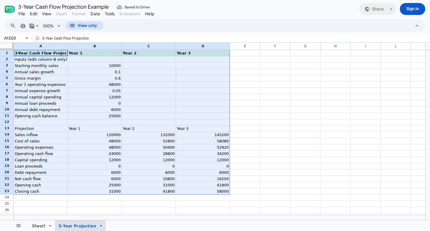
The workbook’s 3-Year Projection sheet uses A1:D23, with columns B through D representing Year 1, Year 2, and Year 3. The model includes:
- Sales inflow
- Cost of sales
- Operating expenses
- Operating cash flow
- Capital spending
- Loan proceeds
- Debt repayment
- Net cash flow
- Opening and closing cash
This is a planning model, not a full accounting cash flow statement. It excludes taxes, working-capital timing, interest, financing fees, and monthly seasonality.
Enter the assumptions
Edit only B3:B11. Enter percentage assumptions as decimals, such as 0.10 for 10%. Capital spending and debt repayment should be positive amounts because the formulas subtract them.
| Cell | Assumption | Illustrative input |
|---|---|---|
| B3 | Starting monthly sales | $10,000 |
| B4 | Annual sales growth | 10% |
| B5 | Gross margin | 60% |
| B6 | Year 1 operating expenses | $48,000 |
| B7 | Annual expense growth | 5% |
| B8 | Annual capital spending | $12,000 |
| B9 | Annual loan proceeds | $0 |
| B10 | Annual debt repayment | $6,000 |
| B11 | Opening cash balance | $25,000 |
Format B4:B5 and B7 as percentages. Format the remaining inputs and B14:D23 as currency or whole numbers.
Keep every input numeric. A text value such as $10k can cause formula errors, so enter 10000 and apply currency formatting instead.
Build the 3-year formulas
Spreadsheet formulas begin with an equals sign and can refer to other cells. For more detail, see the official formula guidance for Google Sheets and Microsoft Excel.
1. Project annual sales
First, convert Year 1 monthly sales into an annual amount. In B14, enter:
=B3*12
Next, enter the following formulas in C14 and D14, respectively, to project Years 2 and 3:
=B14*(1+$B$4)
=C14*(1+$B$4)
The results are $120,000, $132,000, and $145,200.
2. Calculate cost of sales
A 60% gross margin means cost of sales equals 40% of sales. In B15, enter:
=B14*(1-$B$5)
Copy B15 across through D15. The resulting costs are $48,000, $52,800, and $58,080.
3. Grow operating expenses
Year 1 operating expenses come directly from the assumptions. In B16, enter:
=$B$6
To apply 5% annual expense growth, enter the following formulas in C16 and D16, respectively:
=B16*(1+$B$7)
=C16*(1+$B$7)
Operating expenses become $48,000, $50,400, and $52,920.
4. Calculate operating cash flow
Now subtract cost of sales and operating expenses from sales. In B17, enter:
=B14-B15-B16
Copy B17 across through D17. Operating cash flow is $24,000, $28,800, and $34,200.
5. Add investing and financing cash flows
Link the annual capital spending, loan proceeds, and debt repayment assumptions by entering the following formulas in B18, B19, and B20, respectively:
=$B$8
=$B$9
=$B$10
Copy each formula through column D. Then calculate net cash flow by entering this formula in B21:
=B17-B18+B19-B20
Copy B21 across through D21.
The calculation produces:
- Year 1: $24,000 - $12,000 + $0 - $6,000 = $6,000
- Year 2: $28,800 - $12,000 + $0 - $6,000 = $10,800
- Year 3: $34,200 - $12,000 + $0 - $6,000 = $16,200
6. Roll closing cash into the next year
Set Year 1 opening cash equal to the starting balance. In B22, enter:
=$B$11
Each later year begins with the previous year’s closing cash. Enter these formulas in C22 and D22, respectively:
=B23
=C23
Finally, calculate closing cash by adding opening cash and net cash flow. In B23, enter:
=B22+B21
Copy B23 across through D23.
Check the completed projection
Don’t overwrite B14:D23 in the supplied template because those cells contain the projection formulas.
| Projection row | Year 1 | Year 2 | Year 3 |
|---|---|---|---|
| Sales inflow | $120,000 | $132,000 | $145,200 |
| Cost of sales | $48,000 | $52,800 | $58,080 |
| Operating expenses | $48,000 | $50,400 | $52,920 |
| Operating cash flow | $24,000 | $28,800 | $34,200 |
| Capital spending | $12,000 | $12,000 | $12,000 |
| Loan proceeds | $0 | $0 | $0 |
| Debt repayment | $6,000 | $6,000 | $6,000 |
| Net cash flow | $6,000 | $10,800 | $16,200 |
| Opening cash | $25,000 | $31,000 | $41,800 |
| Closing cash | $31,000 | $41,800 | $58,000 |
Use this control check:
Opening cash + net cash flow = closing cash
For Year 3, $41,800 + $16,200 = $58,000. That confirms the cash roll-forward is consistent. The supplied spreadsheet test also matched every formula cell in the baseline case.
Identify a projected funding gap
Review B23:D23. If a closing-cash value is negative, the assumptions create a projected funding gap by the end of that year.
For example, the supplied zero-sales stress case changes only B3 from $10,000 to 0, while all other baseline assumptions remain unchanged.
| Result | Year 1 | Year 2 | Year 3 |
|---|---|---|---|
| Net cash flow | -$66,000 | -$68,400 | -$70,920 |
| Closing cash | -$41,000 | -$109,400 | -$180,320 |
Under this annual model, Year 1 would require at least $41,000 of additional cash to reach a zero year-end balance. The actual funding requirement could be higher if expenses fall due before cash receipts, since the model doesn’t show monthly timing.
For a month-by-month liquidity view, see how to forecast cash runway in Excel or Google Sheets.
Test changes before relying on the projection
As one sensitivity check, change B4 from 10% to 20%. The recorded spreadsheet test produced Year 2 closing cash of $49,000 and Year 3 closing cash of $81,760. Restore B4 to 10% before comparing the workbook with the baseline table.
You should also test these boundaries in a separate copy:
- Set sales growth to 0% and confirm sales remain constant after Year 1.
- Test gross margin at 0% and 100%.
- Set operating expenses, capital spending, debt repayment, or opening cash to zero one at a time.
- Clear each input individually and document the visible result; don’t assume blank inputs are handled safely.
- Paste text into a numeric input and confirm that errors remain visible. Avoid hiding malformed inputs with
IFERRORor converting them to zero withN().
Only the baseline, 20% growth sensitivity, and zero-sales stress case have supplied execution evidence. The remaining checks are recommended tests.
Adapt the projection to your plan
Replace B3:B11 with your operating assumptions, then review:
B17:D17for cash generated by operationsB21:D21for total annual cash generation or burn after capital spending and financingB23:D23for projected year-end liquidity
Keep the units consistent. When monthly sales are entered in B3, multiply by 12 only once. Unless you revise the formulas, enter all other amounts as annual figures.
A positive closing balance means the modeled cash balance stays above zero at each year-end. It doesn’t prove profitability, solvency, or sufficient liquidity within each year.
For a projection connected to income statements and balance sheets, use a 3-statement financial model.
Check the workbook with ModelMonkey
ModelMonkey can inspect spreadsheet context in Google Sheets or Excel and help read ranges, analyze formulas, organize content, or change formatting. After opening the template, you could use this prompt:
Check the formulas in B14:D23 against the assumptions in B3:B11, confirm that opening cash rolls forward once per year, and identify any negative closing-cash values.
Review the assumptions, formulas, and proposed changes before relying on the output. Spreadsheet assistance doesn’t guarantee calculation accuracy.