
=IF(B2="","Blank",IF(COUNTIF($A$2:$A$100,B2)>0,"Yes","No"))
COUNTIF(range, criterion) counts cells that meet a condition. When the count is greater than zero, the value appears in the list. The initial IF prevents an empty input from being classified as missing.
If you need the number of occurrences instead of Yes or No, use:
=IF(B2="",0,COUNTIF($A$2:$A$100,B2))
Microsoft documents the function’s syntax, wildcard criteria, and case-insensitive matching in its COUNTIF function reference.
Supplier-code example
This example checks entered supplier codes against a controlled list. Keep in mind that list membership alone doesn’t prove a supplier or transaction is authorized. It confirms only that the entered text matches a value in the referenced cells.
You can copy the Google Sheets template or download the Excel file.
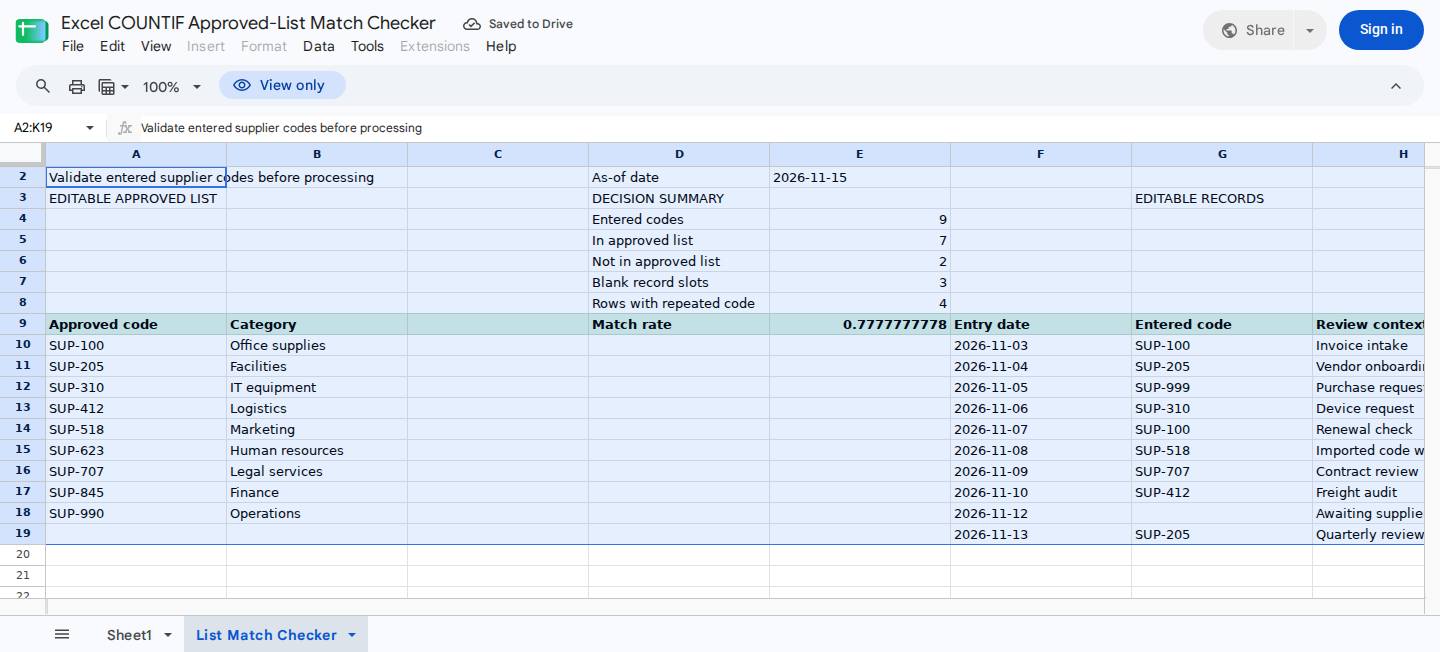
On the List Match Checker sheet:
A10:A18contains the approved codes.B10:B18contains optional categories.F10:F21contains entry dates.G10:G21contains the codes being checked.H10:H21contains review context.I10:I21returns Yes, No, or Blank.J10:J21counts occurrences in the approved list.K10:K21flags duplicates within the entered batch.
The approved list is:
| Cell | Approved code | Category |
|---|---|---|
| A10 | SUP-100 | Office supplies |
| A11 | SUP-205 | Facilities |
| A12 | SUP-310 | IT equipment |
| A13 | SUP-412 | Logistics |
| A14 | SUP-518 | Marketing |
| A15 | SUP-623 | Human resources |
| A16 | SUP-707 | Legal services |
| A17 | SUP-845 | Finance |
| A18 | SUP-990 | Operations |
Return Yes, No, or Blank
Enter this formula in I10 and fill it through I21:
=IF(G10="","Blank",IF(COUNTIF($A$10:$A$18,G10)>0,"Yes","No"))
The dollar signs keep the approved-list range fixed as you copy the formula down. Meanwhile, the reference to G10 changes to G11, G12, and so on.
Expected results include:
SUP-100returnsYes.SUP-999returnsNo.- An empty record cell returns
Blank.
Count approved-list occurrences
To see how many times each entered code appears in the approved list, enter this formula in J10 and fill it through J21:
=IF(G10="",0,COUNTIF($A$10:$A$18,G10))
Interpret the result as follows:
0: The entered value doesn’t appear inA10:A18.1: It appears once.- Above
1: The approved list contains repeated copies of that value.
A zero doesn’t explain why the match failed. The code might be unknown, mistyped, or affected by spaces or other characters.
Flag duplicate entries in the batch
Next, enter this formula in K10 and fill it through K21:
=IF(G10="","Blank",IF(COUNTIF($G$10:$G$21,G10)>1,"Duplicate","Unique"))
Unlike the previous formula, this one counts the current code within the entered batch, not the approved list. When a code occurs twice, both rows are marked Duplicate.
Calculate the batch summary
Use these formulas for the summary in D4:E9:
| Cell | Label | Formula |
|---|---|---|
| E4 | Entered codes | =COUNTIF(G10:G21,"<>") |
| E5 | In approved list | =COUNTIF(I10:I21,"Yes") |
| E6 | Not in approved list | =COUNTIF(I10:I21,"No") |
| E7 | Blank record slots | =COUNTIF(I10:I21,"Blank") |
| E8 | Rows with repeated code | =COUNTIF(K10:K21,"Duplicate") |
| E9 | Match rate | =IF(E4=0,0,E5/E4) |
Format E9 as a percentage. If the entire batch is empty, the zero-denominator condition returns 0.
The baseline batch produces:
| Row | Entered code in G | I: In approved list? | J: List occurrences | K: Batch frequency |
|---|---|---|---|---|
| 10 | SUP-100 | Yes | 1 | Duplicate |
| 11 | SUP-205 | Yes | 1 | Duplicate |
| 12 | SUP-999 | No | 0 | Unique |
| 13 | SUP-310 | Yes | 1 | Unique |
| 14 | SUP-100 | Yes | 1 | Duplicate |
| 15 | SUP-518 with a trailing space | No | 0 | Unique |
| 16 | SUP-707 | Yes | 1 | Unique |
| 17 | SUP-412 | Yes | 1 | Unique |
| 18 | blank | Blank | 0 | Blank |
| 19 | SUP-205 | Yes | 1 | Duplicate |
| 20 | blank | Blank | 0 | Blank |
| 21 | blank | Blank | 0 | Blank |
The control totals are:
- 9 entered codes: 7 matches plus 2 nonmatches.
- 12 record slots: 9 entered codes plus 3 blanks.
- 4 rows containing repeated codes: both occurrences of
SUP-100and both occurrences ofSUP-205. - Match rate:
7 ÷ 9 = 77.78%.
Keep the formulas in every output row, including unused record slots. For example, K18, K20, and K21 return the text Blank; they aren’t empty cells.
These results were recorded using native Google Sheets calculation. The downloadable workbook uses standard Excel formulas, but this specific file wasn’t independently executed in desktop Excel.
Account for COUNTIF wildcards
COUNTIF treats * and ? as wildcard characters. Because the supplier codes above contain neither character, the formulas return the stated results. If your codes might contain wildcards and must be compared literally, use equality comparisons through SUMPRODUCT.
For membership in I10:
=IF(G10="","Blank",IF(SUMPRODUCT(--($A$10:$A$18=G10))>0,"Yes","No"))
For approved-list occurrences in J10:
=IF(G10="",0,SUMPRODUCT(--($A$10:$A$18=G10)))
For batch duplicates in K10:
=IF(G10="","Blank",IF(SUMPRODUCT(--($G$10:$G$21=G10))>1,"Duplicate","Unique"))
Fill each formula through row 21. These versions compare cell values without interpreting * or ? as matching patterns.
Fix apparent matches that return No
In the sample batch, the value in G15 is SUP-518 with a trailing space. It doesn’t equal SUP-518 in the approved list, so the row returns No and 0.
Once you remove the trailing space, the expected results are:
I15:YesJ15:1K15:Unique
The summary then changes to 8 matches, 1 nonmatch, and a match rate of 8 ÷ 9 = 88.89%.
Excel’s TRIM function removes ordinary leading, trailing, and repeated spaces. See Microsoft’s TRIM function documentation.
Whether you should trim automatically depends on the control. Preserving the raw mismatch can help you identify malformed imported codes. Also note that a cell containing only spaces isn’t blank. These formulas classify it as an entered nonmatch rather than Blank.
COUNTIF ignores letter case
COUNTIF isn’t case-sensitive. Changing SUP-100 to sup-100 still matches the approved value and returns an occurrence count of 1.
If uppercase and lowercase codes represent different values, use a case-sensitive comparison method instead. Ordinary COUNTIF isn’t suitable for case-sensitive validation.
Maintain the checker
For each new batch:
- Save a copy first if prior batches must be retained.
- Update the review date in
E2. - Replace only the entries in
F10:H21. - Leave
E4:E9andI10:K21unchanged. - Investigate every
Noresult before relying on the comparison.
The template supports 9 approved-list rows and 12 record rows. If the approved list extends beyond A18 or the batch extends beyond row 21, expand all applicable ranges and fill the row formulas into the added records.
These formulas use commas as argument separators. If your Excel locale expects semicolons, replace the separating commas with semicolons.
For criteria based on several text fragments rather than list membership, see Excel COUNTIF Contains Multiple Criteria.
Use ModelMonkey for this list check
ModelMonkey can inspect spreadsheet context and help with formulas or data-cleanup tasks in Excel and Google Sheets. For this workbook, you could request:
Compare G10:G21 with the approved codes in A10:A18. Keep blank rows classified as Blank, count approved-list occurrences, and flag codes repeated within the entered batch.
When the workflow presents a preview, review the proposed changes before proceeding. Then check the results for an approved code, a missing code, a duplicate, and a blank row. Spreadsheet assistance doesn’t replace checking the formulas and referenced ranges.