
How to Subtract in Google Sheets
Use =B2-C2 to subtract in Google Sheets, fill the formula down, calculate a total remainder, and fix common sign or input mistakes.
To subtract in Google Sheets, enter =B2-C2, where B2 contains the starting amount and C2 contains the amount you want to subtract. Formulas in Google Sheets begin with an equals sign and can reference values in other cells, as explained in Google Editors Help.
In this guide, you’ll use a monthly budget to calculate the amount remaining in each category and across the overall budget.
What You'll Need
- Access to Google Sheets
- A blank spreadsheet, or Copy this Google Sheets template
- Optional: Download the Excel file
Step-by-Step Guide
Enter the budget and spending amounts
Open the sheet named Budget Subtraction. The example occupies Budget Subtraction!A1:D5:
| Category | Budgeted | Spent | Remaining |
|---|---|---|---|
| Rent | 1200 | 1200 | 0 |
| Groceries | 500 | 340 | 160 |
| Transport | 180 | 95 | 85 |
| Total | 1880 | 1635 | 245 |
These amounts are synthetic and use one consistent currency.
If necessary, replace the category names in A2:A4. Then enter the planned amounts in B2:B4 and actual spending in C2:C4.
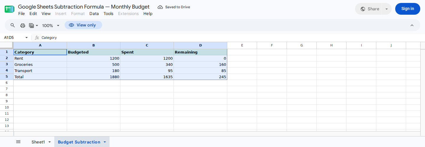
Enter amounts in columns B and C. Column D calculates each difference with a subtraction formula.
Enter and fill down the subtraction formula
Select Budget Subtraction!D2 and enter:
=B2-C2
After you press Enter, Google Sheets performs this calculation:
1200 - 1200 = 0
Next, copy D2 down through D4 by dragging the fill handle or by copying and pasting the cell. Because the formula uses relative cell references, the row numbers adjust automatically:
D2: =B2-C2
D3: =B3-C3
D4: =B4-C4
You should see results of 0, 160, and 85.
Now calculate the totals with:
B5: =SUM(B2:B4)
C5: =SUM(C2:C4)
D5: =B5-C5
The expected total is:
1880 - 1635 = 245
Adding the row-level differences produces the same result:
0 + 160 + 85 = 245
A recorded spreadsheet execution produced these results on 2026-10-17. Two additional checks were also recorded, with each one starting from the original baseline:
- Changing
C3from340to425producedD3=75,C5=1720, andD5=160. - Resetting the baseline, then setting
B4=0andC4=0, producedD4=0,B5=1700,C5=1540, andD5=160.
Separately, an anonymous read of Budget Subtraction!A1:D5 displayed the five rows shown above. This readback confirms the displayed data, but it isn’t a new formula calculation.
Interpret and check the result
Since the formula subtracts spending from the budget:
- A positive result means money remains.
- Zero means the budget and spending are equal.
- A negative result means spending exceeded the budget.
For example, if you set B3 to 500 and C3 to 525, =B3-C3 should return -25. This is a suggested manual check rather than one of the recorded execution cases.
If the result looks wrong, check for these common mistakes:
- Reversed references:
=C3-B3produces the opposite sign from=B3-C3. - Missing equals sign: Entering
B2-C2without=records text instead of starting a formula. - Nonnumeric inputs: When a referenced cell contains text such as
pending, correct the input instead of silently converting it withIFERRORorN. - Blank inputs: Decide whether a blank represents zero or missing data, then test that policy in a copy of the sheet. Blank inputs weren’t covered by the recorded cases.
- Numbers stored as text: Remove leading apostrophes or other characters, then re-enter the value as a number.
You don’t need to worry about comma-versus-semicolon function separators for =B2-C2 because the formula has no function arguments.
ModelMonkey can inspect the active Google Sheets context and help with formula tasks. For this example, you could submit the following request:
Inspect Budget Subtraction!B2:D5. Check that each Remaining cell subtracts Spent from Budgeted on the same row and that D5 equals B5-C5. Show any proposed formula changes for review.
When the workflow presents a preview, review the proposed changes before proceeding. You should also confirm the results against the expected values because formula suggestions may be incorrect.
Wrapping Up
Use =B2-C2 to subtract one Google Sheets cell from another, then fill the formula down to calculate additional rows. In the verified example, subtracting 1635 in spending from a budget of 1880 leaves 245. That amount matches the sum of the category-level differences.
Frequently Asked Questions
How do I subtract the same amount from several cells?
Put the fixed amount in one cell, then use an absolute reference. If the amount is in F1, enter =B2-$F$1 and fill the formula down. The $ signs keep the reference fixed on F1.
Can I subtract more than two cells?
Yes. A formula such as =A1-B1-C1 subtracts B1 and then C1 from A1, working from left to right.
Why is Google Sheets displaying my formula instead of its result?
Check for a leading apostrophe and make sure the cell isn’t formatted as plain text. Select Format > Number > Automatic, remove the apostrophe, and enter the formula again.
What if the result doesn’t update after an input changes?
Confirm that the result cell still contains a formula rather than a pasted value. If the formula remains but the displayed result appears stale, see How to Force Google Sheets to Recalculate Formulas.