
Use an Income and Expense Report Template
Copy an income and expense report template, clean CSV imports, track cash and plans, reconcile records, and roll reports forward.
This income and expense report template tracks cleared and pending cash movements, compares actual expenses with plans, and supports transaction reconciliation. Copy the Google Sheets template or download the Excel file.
The supplied workbook supports 29 transaction rows in A18:J46. For larger imports, this guide includes a Google Sheets staging workflow for up to 10,000 CSV rows. It normalizes dates and whitespace, applies controlled labels, detects duplicate IDs, validates amounts, and identifies unmatched expense categories before loading approved records into an expanded report.
No recorded 10,000-row execution or performance benchmark was supplied. Before using the staging workflow regularly, test it with a representative dirty CSV and check its responsiveness in your working environment. This workbook is a cash activity report, not an accrual-based profit and loss statement.
What You'll Need
- A Google account for Google Sheets, or Microsoft Excel for the supplied 29-row template
- Opening cash across the accounts included in the report
- Income and expense plans for the reporting period
- Transaction dates, amounts, accounts, categories, statuses, and reconciliation results
- A duplicate workbook if you plan to expand the transaction area
- Google Sheets set to the United States locale for the staging formulas in this guide
Step-by-Step Guide
Copy the income and expense report template
Choose either format:
Create 3 copies:
- Baseline: Keep the supplied September example unchanged.
- Verification: Use this copy for the independent checks in this guide.
- Working report: Replace the sample data or add the staging workflow.
Before each independent check, reset the Verification copy from the unchanged Baseline.
The Income & Expense Report sheet contains these areas:
| Range | Purpose |
|---|---|
B4:B9 | Period, opening cash, and overall plans |
E4:E15 | Calculated cash, plan, pending, and reconciliation results |
G5:J14 | Expense-category plans and results |
A18:J46 | Supplied transaction-entry area |
Don’t edit calculated cells in E4:E15, I5:J13, or H14:J14.
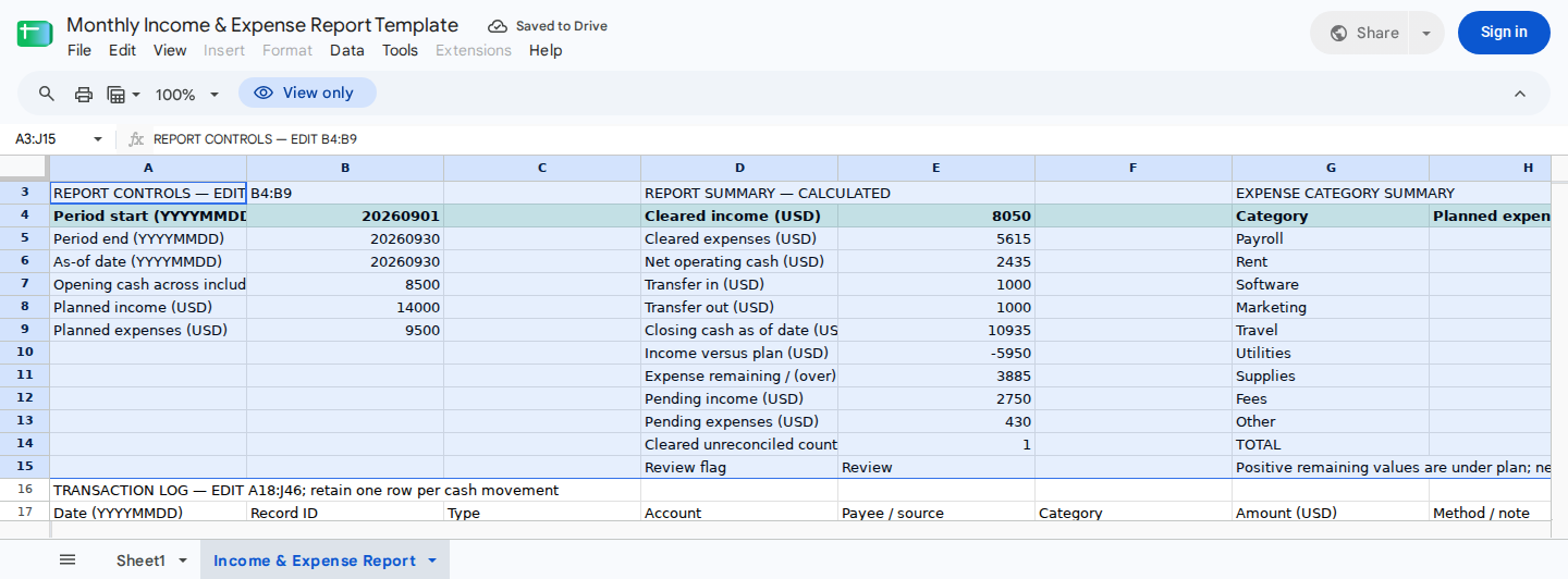
Set the period and plans on the left, then use the central and category summaries to review cash activity, pending amounts, reconciliation exceptions, and spending against plan.
Set the reporting period and plans
In the Working report, replace the sample controls in B4:B9.
The supplied September example uses:
| Cell | Control | Value |
|---|---|---|
B4 | Period start | 20260901 |
B5 | Period end | 20260930 |
B6 | As-of date | 20260930 |
B7 | Opening cash | 8500 |
B8 | Planned income | 14000 |
B9 | Planned expenses | 9500 |
Enter dates as eight-digit YYYYMMDD numbers. The opening cash in B7 should equal the combined opening balances of the cash accounts represented in the transaction log.
Check that:
B4isn’t later thanB5.B6falls within the reporting period.B7:B9contain numbers.- Income and expense plans are zero or greater.
- A zero plan is intentional rather than missing data.
- Every value in
B4:B6represents a real date.
An eight-digit number can still be invalid. For example, 20260931 has the expected length, but September has no 31st day.
In the recorded examples, the as-of date is the month-end date, so B6 equals B5. Interim-date behavior hasn’t been established. Before relying on an interim report, compare it with known transactions at the period start, review date, and period end.
Set expense categories and controlled dropdowns
Enter expense categories in G5:G13 and their planned amounts in H5:H13.
The September example uses:
| Category | Planned expense |
|---|---|
| Payroll | $4,200 |
| Rent | $1,800 |
| Software | $650 |
| Marketing | $800 |
| Travel | $700 |
| Utilities | $450 |
| Supplies | $400 |
| Fees | $200 |
| Other | $300 |
Confirm that H14 shows $9,500, then set B9 to the same amount.
Each category label must contain a value and be unique when capitalization is ignored. Don’t include both Travel and TRAVEL. Case-insensitive criteria could assign one expense to multiple summary rows, which may cause category actuals in I14 to differ from cleared expenses in E5.
Categories in the transaction log must match G5:G13. A misspelling or a hidden, leading, or trailing space can cause an expense to be omitted from its category result.
Don’t use *, ?, or ~ in category names. Their literal treatment hasn’t been verified in the report formulas, so the staging workflow rejects them.
For manual entry, add dropdown validation:
| Range | Allowed values |
|---|---|
C18:C46 | Income, Expense, Transfer In, Transfer Out |
I18:I46 | Cleared, Pending |
J18:J46 | Yes, No |
In Google Sheets, choose Data > Data validation > Add rule > Dropdown and reject invalid entries. In Excel, choose Data > Data Validation > Allow: List.
Dropdowns reduce manual-entry errors, but you still need to audit pasted or imported records. The staging workflow applies case-sensitive checks, so values such as income, cleared, or yes receive REVIEW.
Verify the income and expense report baseline
Keep the synthetic records unchanged in the Baseline copy. Recorded Google Sheets execution with the September controls produced:
| Result | Cell | Expected value |
|---|---|---|
| Cleared income | E4 | $8,050 |
| Cleared expenses | E5 | $5,615 |
| Net operating cash | E6 | $2,435 |
| Transfer in | E7 | $1,000 |
| Transfer out | E8 | $1,000 |
| Closing cash | E9 | $10,935 |
| Income versus plan | E10 | -$5,950 |
| Expense plan remaining | E11 | $3,885 |
| Pending income | E12 | $2,750 |
| Pending expenses | E13 | $430 |
| Cleared unreconciled count | E14 | 1 |
| Review flag | E15 | Review |
The control arithmetic is:
Net operating cash:
$8,050 - $5,615 = $2,435

Closing cash:
$8,500 + $8,050 - $5,615 + $1,000 - $1,000 = $10,935

Income versus plan:
$8,050 - $14,000 = -$5,950

Expense plan remaining:
$9,500 - $5,615 = $3,885
The category totals in H14:J14 should be:
Planned expenses: $9,500
Cleared expenses: $5,615
Remaining:        $3,885
A positive remaining value represents unused expense plan. A negative value means cleared spending is above plan.
If you’re using the Excel download, recalculate the workbook and confirm these values before replacing the sample data.
Enter transactions manually
If your report fits within the supplied range, clear only A18:J29 in the Working report. Keep row 17 and the blank entry rows A30:J46.
Complete one row for each cleared movement or expected pending movement:
| Column | Field | Required entry |
|---|---|---|
A | Date | Numeric YYYYMMDD date |
B | Record ID | Unique identifier |
C | Type | Income, Expense, Transfer In, or Transfer Out |
D | Account | Cash account affected |
E | Payee or source | Counterparty name |
F | Category | Expense category or income label |
G | Amount | USD amount |
H | Note | Explanation or reference |
I | Status | Cleared or Pending |
J | Reconciled | Yes or No |
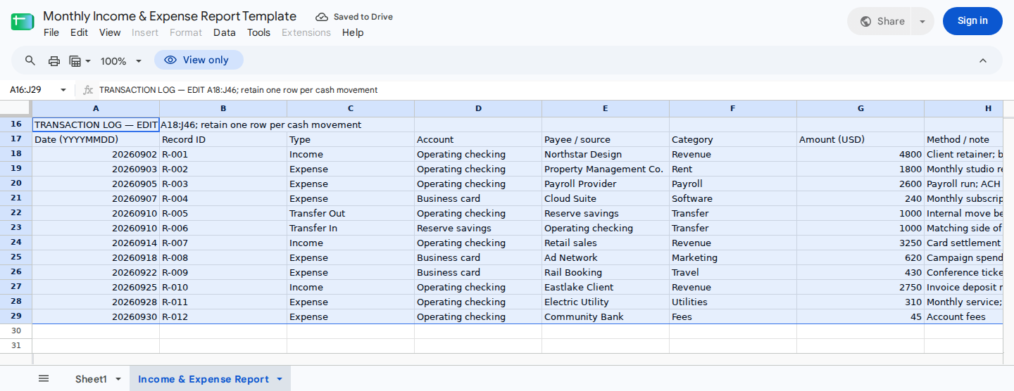
Keep one auditable row for each cash movement. The exact Type, Status, Category, and Reconciled values determine the report results.
Use Cleared only after the movement occurs in the relevant account. Pending amounts appear in E12 or E13 without changing cleared income, cleared expenses, or closing cash.
Record an internal transfer as 2 equal rows:
Transfer Outfrom the source account.Transfer Into the destination account.
Transfers affect E7:E9, but they don’t affect operating income, operating expenses, or expense-category results. The workbook doesn’t confirm that every transfer has a matching second row.
For a correction or refund, add a new row with the original Type and Category. Enter a negative amount and explain it in the Note column. Don’t overwrite an already reconciled record. Zero-value rows have no financial effect, so correct or remove them.
Stage and clean a dirty CSV in Google Sheets
Use a staging sheet when an import contains mixed date formats, blanks, whitespace, duplicate IDs, malformed amounts, or uncontrolled labels. This Google Sheets procedure reserves exactly 10,000 raw rows and doesn’t change the Baseline copy.
Set the required spreadsheet locale
These formulas use commas between arguments. They also assume a period as the decimal separator and commas for thousands, as in 1,234.56.
In the duplicate Working report:
- Choose File > Settings.
- Set Locale to United States.
- Select Save settings and allow the spreadsheet to reload.
- Confirm that entering
1234.56produces a numeric value.
Changing the locale can affect how existing dates and numbers are displayed, so make this change only in the duplicate workbook. If your organization requires another locale, adapt and retest the formula syntax and number-conversion rules.
Create a sheet named Import_Staging with this schema:
| Columns | Contents |
|---|---|
A:J | Raw date, ID, Type, Account, Payee, Category, Amount, Note, Status, Reconciled |
K | Text-date order or native-date confirmation |
L:U | Cleaned versions of the 10 transaction fields |
V | Duplicate-ID result |
W | Date result |
X | Controlled-label result |
Y | Category result |
Z | Load status |
AA1 | Approved-category-list audit |
Paste the CSV headings in row 1 and up to 10,000 data rows in 2:10001.
Preserve raw dates as text
Before importing data, select A2:A10001 and choose Format > Number > Plain text. If you use the Google Sheets file-import dialog, disable Convert text to numbers, dates, and formulas.
Do this before the data enters the sheet. If Google Sheets has already converted 01/09/2026 to a native date, you can’t recover the original DMY-versus-MDY intent from the resulting value. Reload that field from the source as text.
Set a dropdown in K2:K10001 containing exactly YMD, MDY, DMY, and SERIAL, with invalid entries rejected:
YMDfor20260901,2026-09-01, or2026/09/01MDYfor dates such as09/01/2026DMYfor dates such as01/09/2026SERIALonly for a numeric spreadsheet date that you confirmed against the source
Every text date needs the applicable YMD, MDY, or DMY value. If the order is blank, misspelled, or capitalized differently, the normalized date becomes INVALID.
Numeric values from 1 through 99,999 are eligible to be interpreted as spreadsheet date serials only when K contains SERIAL. Selecting SERIAL records that you checked the value against its source. Eight-digit values such as 20260901 should use YMD, not SERIAL.
Normalize dates
Enter this formula in L2. It returns a numeric YYYYMMDD date or INVALID:
=IF(COUNTA(A2:J2)=0,"",
 IFERROR(
  LET(
   raw,TO_TEXT(A2),
   s,TRIM(REGEXREPLACE(CLEAN(
      SUBSTITUTE(
       SUBSTITUTE(
        SUBSTITUTE(
         SUBSTITUTE(raw,CHAR(160)," "),
        UNICHAR(8239)," "),
       UNICHAR(8199)," "),
      UNICHAR(8203),"")
     )," +"," ")),
   nativeCandidate,AND(ISNUMBER(A2),A2>0,A2<100000),
   nativeDate,AND(nativeCandidate,EXACT(K2,"SERIAL")),
   orderOK,OR(EXACT(K2,"YMD"),EXACT(K2,"MDY"),EXACT(K2,"DMY")),
   compact,REGEXMATCH(s,"^[0-9]{8}$"),
   separated,REGEXMATCH(s,"^[0-9]{1,4}[-/.][0-9]{1,2}[-/.][0-9]{1,4}$"),
   digits,REGEXREPLACE(s,"[^0-9]",""),
   parts,SPLIT(REGEXREPLACE(s,"[-.]","/"),"/"),
   y,IF(nativeDate,YEAR(A2),
      IF(compact,
         IF(EXACT(K2,"YMD"),VALUE(LEFT(digits,4)),VALUE(RIGHT(digits,4))),
         IF(EXACT(K2,"YMD"),VALUE(INDEX(parts,1,1)),VALUE(INDEX(parts,1,3))))),
   m,IF(nativeDate,MONTH(A2),
      IF(compact,
         IF(EXACT(K2,"YMD"),VALUE(MID(digits,5,2)),
            IF(EXACT(K2,"MDY"),VALUE(LEFT(digits,2)),VALUE(MID(digits,3,2)))),
         IF(EXACT(K2,"YMD"),VALUE(INDEX(parts,1,2)),
            IF(EXACT(K2,"MDY"),VALUE(INDEX(parts,1,1)),VALUE(INDEX(parts,1,2)))))),
   d,IF(nativeDate,DAY(A2),
      IF(compact,
         IF(EXACT(K2,"YMD"),VALUE(RIGHT(digits,2)),
            IF(EXACT(K2,"MDY"),VALUE(MID(digits,3,2)),VALUE(LEFT(digits,2)))),
         IF(EXACT(K2,"YMD"),VALUE(INDEX(parts,1,3)),
            IF(EXACT(K2,"MDY"),VALUE(INDEX(parts,1,2)),VALUE(INDEX(parts,1,1)))))),
   dt,DATE(y,m,d),
   IF(
    AND(
     OR(nativeDate,AND(orderOK,OR(compact,separated))),
     YEAR(dt)=y,
     MONTH(dt)=m,
     DAY(dt)=d
    ),
    VALUE(TEXT(dt,"yyyymmdd")),
    "INVALID"
   )
  ),
  "INVALID"
 ))
For text dates, the component checks reject impossible dates such as September 31. Numeric serials pass only when the value is within the specified range and K contains the exact SERIAL confirmation.
Clean text fields
Enter this formula in M2, then fill it right through Q2. The relative source reference changes from B2 through F2:
=IF(COUNTA($A2:$J2)=0,"",
 LET(
  s,TO_TEXT(B2),
  normalized,
   SUBSTITUTE(
    SUBSTITUTE(
     SUBSTITUTE(
      SUBSTITUTE(s,CHAR(160)," "),
     UNICHAR(8239)," "),
    UNICHAR(8199)," "),
   UNICHAR(8203),""),
  TRIM(REGEXREPLACE(CLEAN(normalized)," +"," "))
 ))
Enter the same pattern in S2, referencing H2, then fill it right through U2:
=IF(COUNTA($A2:$J2)=0,"",
 LET(
  s,TO_TEXT(H2),
  normalized,
   SUBSTITUTE(
    SUBSTITUTE(
     SUBSTITUTE(
      SUBSTITUTE(s,CHAR(160)," "),
     UNICHAR(8239)," "),
    UNICHAR(8199)," "),
   UNICHAR(8203),""),
  TRIM(REGEXREPLACE(CLEAN(normalized)," +"," "))
 ))
These formulas normalize repeated ordinary spaces, ASCII control characters, nonbreaking spaces, narrow nonbreaking spaces, figure spaces, and zero-width spaces. Inspect other unfamiliar source-system characters before approving the import.
Validate and convert amounts
Enter this formula in R2:
=IF(COUNTA($A2:$J2)=0,"",
 LET(
  raw,TO_TEXT(G2),
  s,TRIM(REGEXREPLACE(CLEAN(
     SUBSTITUTE(
      SUBSTITUTE(
       SUBSTITUTE(
        SUBSTITUTE(raw,CHAR(160)," "),
       UNICHAR(8239)," "),
      UNICHAR(8199)," "),
     UNICHAR(8203),"")
    )," +"," ")),
  valid,
   REGEXMATCH(
    s,
    "^(-?\$?([0-9]+|[0-9]{1,3}(,[0-9]{3})+)(\.[0-9]{1,2})?|\(\$?([0-9]+|[0-9]{1,3}(,[0-9]{3})+)(\.[0-9]{1,2})?\))$"
   ),
  IF(
   NOT(valid),
   "INVALID",
   IF(
    LEFT(s,1)="(",
    -VALUE(REGEXREPLACE(s,"[\$(),]","")),
    VALUE(SUBSTITUTE(SUBSTITUTE(s,"$",""),",",""))
   )
  )
 ))
Under the United States locale, this accepts unsigned amounts, leading-minus negatives, optional dollar signs, comma-separated thousands, up to 2 decimal places, and accounting negatives such as (430) or ($430). It rejects malformed strings such as 12abc34.
Negative corrections and refunds remain valid numeric movements. Zero amounts are rejected later because they don’t provide evidence of cash activity.
Add duplicate, label, and category checks
Use this formula in V2 to find duplicate IDs. It escapes wildcard characters in the ID:
=IF(M2="","",
IF(
COUNTIF(
$M$2:$M$10001,
"="®EXREPLACE(M2,"([~*?])","~$1")
)>1,
"DUPLICATE",
""
))
COUNTIF performs this duplicate check without case sensitivity. Resolve IDs that differ only by capitalization against the source system.
Next, use this formula in W2 to flag missing, invalid, or unconfirmed dates:
=IF(COUNTA(A2:J2)=0,"",
 IF(
  OR(
   L2="",
   L2="INVALID",
   AND(ISNUMBER(A2),A2>0,A2<100000,NOT(EXACT(K2,"SERIAL")))
  ),
  "BAD DATE",
  ""
 ))
Use EXACT in X2 to enforce the documented spelling and capitalization:
=IF(COUNTA(A2:J2)=0,"",
 TEXTJOIN(", ",TRUE,
  IF(
   NOT(OR(
    EXACT(N2,"Income"),
    EXACT(N2,"Expense"),
    EXACT(N2,"Transfer In"),
    EXACT(N2,"Transfer Out")
   )),
   "TYPE",
   ""
  ),
  IF(
   NOT(OR(EXACT(T2,"Cleared"),EXACT(T2,"Pending"))),
   "STATUS",
   ""
  ),
  IF(
   NOT(OR(EXACT(U2,"Yes"),EXACT(U2,"No"))),
   "RECONCILED",
   ""
  )
 ))
Then use this formula in Y2 to check expense categories with case-sensitive equality:
=IF(EXACT(N2,"Expense"),
 IF(
  REGEXMATCH(Q2,"[~*?]"),
  "PROHIBITED CATEGORY CHARACTER",
  IF(
   SUM(ARRAYFORMULA(N(EXACT(
    Q2,
    'Income & Expense Report'!$G$5:$G$13
   ))))=0,
   "UNMATCHED CATEGORY",
   ""
  )
 ),
 "")
Enter this approved-category-list audit in AA1:
=LET(
 categories,'Income & Expense Report'!G5:G13,
 cleaned,
  ARRAYFORMULA(
   TRIM(
    REGEXREPLACE(
     CLEAN(
      SUBSTITUTE(
       SUBSTITUTE(
        SUBSTITUTE(
         SUBSTITUTE(categories,CHAR(160)," "),
        UNICHAR(8239)," "),
       UNICHAR(8199)," "),
      UNICHAR(8203),"")
     ),
     " +"," "
    )
   )
  ),
 normalized,ARRAYFORMULA(LOWER(cleaned)),
 hasBlank,SUM(ARRAYFORMULA(N(cleaned="")))>0,
 hasWhitespace,SUM(ARRAYFORMULA(N(categories<>cleaned)))>0,
 hasWildcard,SUM(ARRAYFORMULA(N(REGEXMATCH(cleaned,"[~*?]"))))>0,
 hasDuplicate,COUNTUNIQUE(normalized)<>ROWS(categories),
 IF(
  hasBlank,
  "REVIEW BLANK CATEGORIES",
  IF(
   hasWhitespace,
   "REVIEW CATEGORY WHITESPACE",
   IF(
    hasWildcard,
    "REVIEW CATEGORY CHARACTERS",
    IF(
     hasDuplicate,
     "REVIEW DUPLICATE CATEGORIES",
     "OK"
    )
   )
  )
 )
)
This audit cleans the category labels before checking for blanks and duplicates. As a result, a cell containing only spaces returns REVIEW BLANK CATEGORIES, not OK. It also flags category cells whose raw value differs from the cleaned value.
Finally, enter this row-level decision formula in Z2:
=IF(COUNTA(A2:J2)=0,"",
 IF(OR(
   COUNTBLANK(L2:U2)>0,
   V2<>"",
   W2<>"",
   X2<>"",
   Y2<>"",
   R2="INVALID",
   R2=0,
   AND(ISNUMBER(A2),A2>0,A2<100000,NOT(EXACT(K2,"SERIAL")))
 ),
 "REVIEW",
 "READY"))
Fill L2:Z2 through row 10001. A raw row containing only whitespace remains active, but cleanup exposes the missing fields and gives it REVIEW.
Create a separate sheet named Import_Audit. Put Unmatched categories in A1, then enter this formula in Import_Audit!A2:
=IFNA(
 SORT(
  UNIQUE(
   FILTER(
    Import_Staging!Q2:Q10001,
    Import_Staging!Y2:Y10001="UNMATCHED CATEGORY",
    Import_Staging!Q2:Q10001<>""
   )
  )
 ),
 "No unmatched categories"
)
The qualified ranges ensure that the formula audits Import_Staging, regardless of its destination. When there are no matches, it returns the scalar message No unmatched categories.
The Excel download supports the original manual workflow. This guide doesn’t provide equivalent Excel or Power Query transformations for these staging rules.
Expand the income and expense report for 10,000 rows
The supplied report stops at row 46, so make these changes only in a duplicate workbook.
For a 10,000-row Google Sheets version:
- Insert
9,971rows above row 47. The expanded transaction area becomesA18:J10017. - Clear the existing synthetic transactions from the expanded area.
- Update every direct transaction range ending at row 46 so it ends at row 10017.
- Inspect the formulas in
E4:E5,E7:E8,E12:E14, andI5:I13, which are the documented cells using transaction ranges. - Keep derived calculation cells such as
E6,E9:E11,E15, andJ5:J14intact. - Enter the following loader formula in
A18.
=LET(
 activeFlags,
  BYROW(
   Import_Staging!A2:J10001,
   LAMBDA(rowData,COUNTA(rowData)>0)
  ),
 allowedDispositionFlags,
  MAP(
   Import_Staging!Z2:Z10001,
   LAMBDA(disposition,
    OR(
     EXACT(disposition,"READY"),
     EXACT(disposition,"REVIEW")
    )
   )
  ),
 hasDispositionFlags,
  MAP(
   Import_Staging!Z2:Z10001,
   LAMBDA(disposition,disposition<>"")
  ),
 missingAllowedDisposition,
  SUM(
   N(activeFlags)*
   (1-N(allowedDispositionFlags))
  ),
 inactiveWithDisposition,
  SUM(
   (1-N(activeFlags))*
   N(hasDispositionFlags)
  ),
 reviewRows,
  COUNTIF(Import_Staging!Z2:Z10001,"REVIEW"),
 IF(
  OR(
   Import_Staging!AA1<>"OK",
   reviewRows>0,
   missingAllowedDisposition>0,
   inactiveWithDisposition>0
  ),
  "",
  IFNA(
   FILTER(
    Import_Staging!L2:U10001,
    Import_Staging!Z2:Z10001="READY"
   ),
   ""
  )
 ))
Keep A18:J10017 otherwise empty so the formula can expand.
The load is all or nothing. The report remains blank when:
Import_Staging!AA1doesn’t returnOK.- Any active staging row has
REVIEWin columnZ. - Any active raw row lacks an exact
READYorREVIEWdisposition. - Any inactive raw row has a value in column
Z.
The last 2 checks apply to individual rows. A disposition on an inactive row can’t offset a missing disposition on an active row.
When there are no source rows, the loader returns a scalar blank instead of a filter error. Once the category audit passes and every active row is READY, it returns the cleaned transaction columns from L:U.
Because the loader populates the report range, maintain dropdown values, corrections, status changes, and reconciliation values in Import_Staging. Don’t type inside the populated range.
Reconcile cleared and pending items
During each review:
- Update the as-of date in
B6. - Add new manual records or replace the staging import.
- Compare each cleared record with the applicable account statement.
- Change Reconciled to
Yesonly after the movement matches. - Change a pending record to
Clearedonly after it occurs. - Review
E14andE15.
For a manual report, update Status in column I and Reconciled in column J. For a staged report, update the corresponding raw values in Import_Staging!I:J. The cleaned values in T:U and the loaded report will then refresh.
In the recorded month-end setup, E14 counts in-period cleared records still marked No. Cell E15 displays Review when that count is greater than zero or closing cash is negative.
To reproduce the September status transition, reset the Verification copy from the unchanged Baseline. Then:
- Change
I26fromPendingtoCleared. - Change
J26fromNotoYes.
This clears and reconciles the $430 Travel expense. Confirm:
| Result | Cell | Expected value |
|---|---|---|
| Cleared expenses | E5 | $6,045 |
| Net operating cash | E6 | $2,005 |
| Closing cash | E9 | $10,505 |
| Expense plan remaining | E11 | $3,455 |
| Pending expenses | E13 | $0 |
| Travel actual | I9 | $430 |
| Travel remaining | J9 | $270 |
E14 remains 1, and E15 remains Review, because another cleared transaction is still unreconciled. Reset the Verification copy again before performing the October check.
Test the 10,000-row staging workflow
No recorded 10,000-row execution or timing benchmark was supplied for this workbook. Before regular use, run this acceptance check on a duplicate containing the dirty 10,000-row CSV your team receives. Preserve its mixed dates, blanks, whitespace, duplicates, and unexpected categories during the test.
Put the acceptance formulas on the separate Import_Audit sheet so they can’t overwrite staging or report data.
Add row-count and disposition controls
Put Active raw rows in Import_Audit!B1, then enter this formula in B2:
=SUM(BYROW(
 Import_Staging!A2:J10001,
 LAMBDA(rowData,N(COUNTA(rowData)>0))
))
This counts each row containing any raw value, including whitespace-only text, once.
Put Active rows without allowed disposition in Import_Audit!C1, then enter this formula in C2:
=LET(
 activeFlags,
  BYROW(
   Import_Staging!A2:J10001,
   LAMBDA(rowData,COUNTA(rowData)>0)
  ),
 allowedDispositionFlags,
  MAP(
   Import_Staging!Z2:Z10001,
   LAMBDA(disposition,
    OR(
     EXACT(disposition,"READY"),
     EXACT(disposition,"REVIEW")
    )
   )
  ),
 SUM(
  N(activeFlags)*
  (1-N(allowedDispositionFlags))
 )
)
Cell C2 must return 0.
Put Inactive rows with disposition in Import_Audit!D1, then enter this formula in D2:
=LET(
 activeFlags,
  BYROW(
   Import_Staging!A2:J10001,
   LAMBDA(rowData,COUNTA(rowData)>0)
  ),
 hasDispositionFlags,
  MAP(
   Import_Staging!Z2:Z10001,
   LAMBDA(disposition,disposition<>"")
  ),
 SUM(
  (1-N(activeFlags))*
  N(hasDispositionFlags)
 )
)
Cell D2 must also return 0.
Put Review rows in Import_Audit!E1, then enter this formula in E2:
=COUNTIF(Import_Staging!Z2:Z10001,"REVIEW")
Resolve every issue against the source data until E2 returns 0. The loader also requires Import_Staging!AA1 to return OK.
Add month-end control totals
Enter these exact Type criteria in Import_Audit!F1:I1:
| Cell | Value |
|---|---|
F1 | Income |
G1 | Expense |
H1 | Transfer In |
I1 | Transfer Out |
Enter this formula in Import_Audit!F2, then fill it right through I2:
=SUMIFS(
 Import_Staging!$R$2:$R$10001,
 Import_Staging!$N$2:$N$10001,F$1,
 Import_Staging!$T$2:$T$10001,"Cleared",
 Import_Staging!$Z$2:$Z$10001,"READY",
 Import_Staging!$L$2:$L$10001,">="&'Income & Expense Report'!$B$4,
 Import_Staging!$L$2:$L$10001,"<="&'Income & Expense Report'!$B$5
)
Each cell tests one exact intended Type separately. Rows reach READY only after the case-sensitive Type and Status checks pass.
For the month-end setup where B6 equals B5, compare:
| Audit cell | Report cell |
|---|---|
Import_Audit!F2 | E4 |
Import_Audit!G2 | E5 |
Import_Audit!H2 | E7 |
Import_Audit!I2 | E8 |
Also confirm:
- Category actuals in
I14equal cleared expenses inE5. - Closing cash equals opening cash plus net operating cash plus Transfer In minus Transfer Out.
- Rows dated exactly on
B4andB5are included. - Rows before
B4or afterB5don’t affect the period totals.
The supplied execution evidence covers month-end reporting only. Keep B6 equal to B5 for these acceptance controls.
Check dirty-data behavior
In a separate acceptance copy, confirm that:
- Raw dates remain text unless they are confirmed native date serials.
- Every text date has an exact
YMD,MDY, orDMYvalue in columnK. - A blank or invalid date order produces
INVALIDinL,BAD DATEinW, andREVIEWinZ. - A numeric date serial without exact
SERIALconfirmation receivesREVIEW. - An impossible date such as
20260931receivesREVIEW. 1,234.56becomes the numeric value1234.56.(430)becomes-430.12abc34becomesINVALID.- A zero amount receives
REVIEW. - A whitespace-only raw row remains active and receives
REVIEW. - Lowercase controlled labels such as
incomeorclearedreceiveREVIEW. - Duplicate IDs are reported even when they contain
*,?, or~. - Duplicate IDs are resolved against the source system rather than deleted automatically.
- Expense categories containing
*,?, or~receiveREVIEW. - An expense category not found in
G5:G13appears in the unmatched-category report. - A category cell containing only spaces makes
AA1returnREVIEW BLANK CATEGORIES. - A category with leading or trailing whitespace makes
AA1returnREVIEW CATEGORY WHITESPACE. - Category names differing only by capitalization make
AA1returnREVIEW DUPLICATE CATEGORIES. - An empty import returns a blank report area rather than a filter error.
- Matching
Transfer OutandTransfer Inrows affectE7:E9but not operating or category totals. - A negative correction using the original Type and Category reverses the applicable amount without overwriting the reconciled source row.
- A row below the expanded range is excluded until every affected staging, loader, and report range is extended.
Keep the formulas bounded to the required capacity. Check recalculation, filtering, scrolling, and editing responsiveness in the browser, spreadsheet application, and hardware your team uses. The 10,000-row range defines capacity. It isn’t evidence of a performance result.
If the source exceeds 10,000 rows, extend the staging, report, loader, audit, and control ranges together. Then rerun every acceptance check.
ModelMonkey can inspect spreadsheet ranges and help identify inconsistent labels or formula errors in Google Sheets or Excel. For this workflow, use a read-only request such as:
Without changing cells, inspect Import_Staging!A2:AA10001,
Import_Audit!A1:I2, and the 'Income & Expense Report' sheet.

Report:
- active raw rows in A:J without an exact READY or REVIEW result in Z
- inactive raw rows in A:J that have any value in Z
- active rows with missing cleaned fields in L:U
- duplicate cleaned record IDs in M
- INVALID or blank normalized dates in L
- text-date rows whose K value is not exactly YMD, MDY, or DMY
- numeric native-date serials whose K value is not exactly SERIAL
- values outside the documented Type, Status, and Reconciled lists
- Expense categories in Q that do not exactly match G5:G13
- blank, whitespace-only, or duplicate category labels in G5:G13
- category labels containing *, ?, or ~
- zero or nonnumeric cleaned amounts in R
- rows marked REVIEW in Z
- formula errors in the report summary
- any difference between cleared expenses in E5 and category actuals in I14

Give the row or cell address for every finding. Do not correct source
records or remove duplicates.
Review each finding against source records and account statements. If you ask ModelMonkey to correct cells, review the proposed changes when the workflow presents a preview. Spreadsheet assistance doesn’t replace reconciliation or guarantee that every result is correct.
Roll the income and expense report forward
Monthly rollover is manual. Finish reconciling the current month, archive a copy, and record the verified closing cash from E9.
To reproduce the recorded October continuation case, reset the Verification copy from the unchanged September Baseline. Set:
B4to20261001B5to20261031B6to20261031B7to10935
For this independent check, retain the September plans:
- Leave
B8at14000. - Leave
B9at9500. - Leave
H5:H13unchanged.
The retained category plans are:
| Cell | Value |
|---|---|
H5 | 4200 |
H6 | 1800 |
H7 | 650 |
H8 | 800 |
H9 | 700 |
H10 | 450 |
H11 | 400 |
H12 | 200 |
H13 | 300 |
Cell H14 should remain $9,500.
Enter this complete record in A30:J30:
20261002 | R-013 | Income | Operating checking | Harbor Client | Revenue | 1500 | Project deposit; bank transfer | Cleared | Yes
The exact cells are:
| Cell | Value |
|---|---|
A30 | 20261002 |
B30 | R-013 |
C30 | Income |
D30 | Operating checking |
E30 | Harbor Client |
F30 | Revenue |
G30 | 1500 |
H30 | Project deposit; bank transfer |
I30 | Cleared |
J30 | Yes |
The October date criteria exclude the retained September transactions. Opening cash is carried into B7 once, so the old transactions aren’t counted again.
Confirm:
| Result | Cell | Expected value |
|---|---|---|
| Cleared income | E4 | $1,500 |
| Cleared expenses | E5 | $0 |
| Net operating cash | E6 | $1,500 |
| Closing cash | E9 | $12,435 |
| Pending income | E12 | $0 |
| Pending expenses | E13 | $0 |
| Review flag | E15 | OK |
The closing-cash check is:
$10,935 opening cash + $1,500 cleared income = $12,435
For an actual rollover, replace the retained September plans with the new month’s values in B8:B9 and H5:H13. The workbook doesn’t carry balances forward automatically or connect to a bank account.
Wrapping Up
The income and expense report template shows cleared income, expenses, transfers, pending items, closing cash, and category-plan variances for a monthly reporting period. The supplied September example closes at $10,935, has $3,885 of expense plan remaining, and flags one cleared unreconciled record.
Use the original A18:J46 area for small reports. For a dirty CSV, work in a duplicate Google Sheets workbook. Preserve raw dates, clean whitespace, resolve duplicate IDs and unmatched categories, and require every row audit to pass before loading records.
Before using the expanded version regularly, test it with your own 10,000-row CSV and working environment. For related workflows, see Freelance Expense Tracking in Google Sheets and How to Forecast Freelance Income and Expenses.
Frequently Asked Questions
Is this income and expense report a profit and loss statement?
No. It’s a cash activity report based on cleared and pending transactions. It doesn’t account for accruals, depreciation, receivables, liabilities, or other adjustments used in a formal profit and loss statement.
Why is a transaction missing from the totals?
Check its date, Type, Status, amount, and expense Category. A record can be omitted when its controlled label doesn’t match, its date is outside the reporting period, or its category doesn’t match G5:G13.
For staged data, also check for blank required fields, hidden whitespace, a zero or malformed amount, a duplicate ID, an unconfirmed date serial, REVIEW in column Z, or a formula range that ends before the record.
Why must the staging workbook use the United States locale?
The supplied Google Sheets formulas parse amounts with period decimals and comma thousands separators, such as 1,234.56. Another locale may use different formula separators or interpret that amount differently.
If you must retain another locale, adapt and retest both the formula syntax and amount-conversion rules.
How does the staging sheet handle mixed date formats?
Format raw column A as plain text before importing, then assign each text date an exact YMD, MDY, or DMY value in column K. The normalization formula converts valid dates to numeric YYYYMMDD values and marks missing, misspelled, or calendar-invalid inputs as INVALID.
For a confirmed numeric spreadsheet date, use SERIAL. Without that confirmation, the row receives REVIEW.
Why must category labels be unique and free of whitespace?
Duplicate category labels can make one expense appear in multiple category rows. Leading, trailing, or hidden whitespace can prevent an otherwise correct category from matching.
The category audit cleans the labels before checking for blanks and duplicates. It blocks loading when a category is empty, contains only spaces, needs whitespace cleanup, uses prohibited characters, or duplicates another category without regard to capitalization.
Are controlled labels case-sensitive?
The original workbook’s case-matching behavior hasn’t been established. The staging audit uses case-sensitive checks: Income, Cleared, and Yes pass, while income, cleared, and yes receive REVIEW.
Should pending invoices affect closing cash?
No. In the recorded month-end setup, pending items appear in E12 or E13 without changing cleared income, cleared expenses, or closing cash. Change a record to Cleared only after its cash movement occurs.
How should I record an internal transfer?
Enter an equal Transfer Out from the source account and Transfer In to the destination account. The report shows both sides separately but doesn’t automatically create or match the pair.
Can I add transactions below row 46?
Only after modifying a duplicate workbook. The supplied formula ranges don’t expand automatically. Extend the transaction area and every affected formula, loader, staging, and audit range together, then compare the results with independent control totals.
Has the template been performance-tested with 10,000 rows?
No recorded 10,000-row execution or benchmark was supplied. The staging workflow provides bounded ranges and acceptance controls for evaluating a dirty 10,000-row CSV in your environment. Check recalculation and editing responsiveness before regular use.
Can I use the 10,000-row staging workflow in Excel?
The supplied Excel file supports the original manual template workflow. The staging formulas in this guide are specific to Google Sheets. An equivalent Excel or Power Query process would require separately defined and validated transformations.
Does the template import bank transactions automatically?
No. Transactions, reconciliation changes, and monthly rollover must be entered manually or loaded through the staging workflow. The workbook doesn’t connect to a bank account.